Transformerの計算量は入力系列の長さの二乗に比例することから長い系列を取り扱う際に計算コストの課題が生じます。当記事ではこのような課題の解決にあたって用いられるSparse Attentionの分類とそれぞれの研究例について確認を行います。A Survey of Transformers 」やそれぞれの論文を参考にしました。
・用語/公式解説https://www.hello-statisticians.com/explain-terms
Sparse Attention Sparse Attentionの概要 Transformerでは$Q K^{\mathrm{T}}$の計算に基づいてAttention Matrixの計算を行うが、このAttention Matrixの行列のサイズは系列の長さの二乗となり、計算コストが大きい。
このような際にAttention Matrixを疎行列で置き換える手法をSparse Attentionという。Aparse Attentionの活用にあたっては「どのような疎行列で表せば効率良く近似できるか」などを重視すると理解しやすい。
Sparse Attentionの分類 Sparse Attentionを実現する方法は「位置に基づく疎行列の作成」と「隠れ層のベクトルの類似度に基づく疎行列の作成」の二つに大別することができる。
当記事ではSurvey論文を元に位置に基づくSparse Attentionを「Position-based Sparse Attention」、隠れ層のベクトルの類似度に基づくSparse Attentionを「Content-based Sparse Attention」と表し、次節と次々節でそれぞれ取り扱う。
Position-based Sparse Attention 基本パターン 下図を元にPosition-based Sparse Attentionを構成する$5$つのパターンを確認することができる。
A Survey of TransformerのFig.$4$ 図の上側が$l$層から$l+1$層を計算するにあたってのAttentionの重みが$0$かどうかを表し、下側がAttention Matrixの数値に対応する($0$の場合白、$0$以外の場合色付けされる)。上側が特殊な形式のグラフ、下側が隣接行列であると解釈することもできる。
以下で取り扱うStar-Transformer、Longformer、ETC、BigBirdなどの研究ではそれぞれこの基本パターンの組み合わせによってSparse Attentionを構成する。
基本パターンの解釈 基本パターンの解釈を以下にまとめた。
global 特定のトークン(ノード)を全てのトークンのAttention計算に用いるかつ、特定のトークンのAttention計算には全てのトークンの隠れ層を用いる。 band 近隣のトークンのみを用いてAttention計算を行う。CNNとRNNはbandの特殊な例であると解釈することもできる。 dilated bandによる局所処理のreceptive field(特定の位置の出力を構成する入力領域)を広げるにあたって用いられる処理。詳しくはWaveNet論文などを参照すると良い。 random ランダムなグラフは完全グラフ(通常のTransformer)と似た性質を持つことを活用。 block local 入力をセグメント単位に分けてAttention計算を行う。
Star-Transformer A Survey of Transformer ではStar-Transformerが下記のような図で表される。
A Survey of Transformer:Fig.$5$.(a) 上図より、Star-Transformerが「global attention」と「band attention」の組み合わせであることが確認できる。
Longformer A Survey of Transformer ではLongformerが下記のような図で表される。
A Survey of Transformer:Fig.$5$.(b) 上図より、Star-Transformerが「global attention」と「band attention」の組み合わせであることが確認できる。
Longformer論文 Figure$\, 2$ また、上図で表されるLongformer論文のFigure$\, 2$より、Attention Matrixの詳細が確認できる。Surveyでは「global」+「band」のみが記載されているが、Longformer論文では「global」+「dilated」のパターンも記載されている。
ETC A Survey of TransformerではETC(Extended Transformer Construction)が下記のような図で表される。
A Survey of Transformer:Fig.$5$.(c) 上図より、ETCがStar-Transformerと同様に「global attention」と「band attention」の組み合わせであることが確認できる。
BigBird A Survey of TransformerではBig Birdが下記のような図で表される。
A Survey of Transformer:Fig.$5$.(d) 上図より、Big Birdが「global attention」+「band attention」+「random attention」であることが確認できる。
Big Bird論文 Figure$\, 1$ また、Big Bird論文 でもSurveyと同様な図が確認できる。色遣いが近いことから、Surveyの図はBig Birdをある程度参考に作成したことが推察される。
Content-based Sparse Attention Content-based Sparse Attentionでは隠れ層のベクトルの値に基づいてAttention Matrixを疎行列で表す手法である。以下、LSH(locality-sensitive hashing)を用いるReformerやRouting Transformerなどの具体的な研究例について確認を行う。
Reformer ReformerはLSH(locality-sensitive hashing)に基づくLSH AttentionというSparse Attentionを行う。以下、LSHとLSH Attentionについて確認を行う。
locality-sensitive hashing
次元$d_{k}$のベクトル$\mathbf{x} \in \mathbb{R}^{d_{k}}$を$b$値に分類するハッシュ関数を$h$とおく。このとき$h(\mathbf{x}) \in \{1, 2, \cdots, b \}$である。
Reformer論文では乱数に基づく行列$R \in \mathbb{R}^{d_{k} \times b/2}$に基づいてハッシュ関数$h$を定める。ハッシュ関数の定義にあたって、$[\mathbf{u}; \mathbf{v}]$をベクトル$\mathbf{u}$と$\mathbf{v}$の連結(concatnation)であると定義する。
このときハッシュ関数$h(\mathbf{x})$を下記のように定義する。
上記の$\mathbf{x}R$が要素数$\displaystyle \frac{b}{2}$のベクトルであるので、ハッシュ関数$h$は要素数$b$のベクトル$[\mathbf{x}R; -\mathbf{x}R]$から最大値を持つインデックスを選択する関数であると解釈できる。
locality-sensitive hashingでは行列$R$がランダムにベクトルを回転させる行列であると解釈することもできるので、直感的には下図のような図を元に理解しておくとと良い。
Reformer論文 Figure$\, 1$ ReformerにおけるLSH Attentionは当項で確認を行なったハッシュ関数$h$に基づくlocality-sensitive hashingを用いたSparse Attentionである。
LSH Attention
LSH AttentionではTransformerのself-Attentionの式を下記のように改変を行う。
上記の理解にあたっては$\mathcal{P}_{i}$が「位置$i$のqueryである$q_{i}$が類似する位置の集合」であることに着目することが重要である。また、$z$は分配関数(partition function)であり、ソフトマックス関数と同様に出力の正規化を行う関数である。
LSH Attentionでは集合$\mathcal{P}_{i}$を前項で定義したハッシュ関数$h$を用いて下記のように定義する。
上記は「位置$i$に対して$h(q_{i}) = h(k_{j})$が成立する位置$j$の集合を$\mathcal{P}_{i}$と定義する」と解釈することができる。
Routing Transformer Routing Transformerではクラスタリングと同様の枠組みを用いてSparse Attention処理を行う。以下、クラスタリングに基づくSparse Attentionの計算とクラスタリングに用いるCentroid vectorsの計算について確認する。
Routing Attention
Routing Transformer論文では下記のような式でSparse Attentionの計算を行う。
上記の式はRouting Transformer論文の$(8)$式に改変を行なったものである。$A$はAttention Matrix、$i$は位置$i$のインデックス、$j$はAttention処理後の位置$i$の隠れ層を計算するにあたって用いる位置$j$のインデックスをそれぞれ表す。$j$は$A$の列に対応する一方で、$V$の行に対応することに注意が必要である。 また、$X_{i}’$はFFN層の入力に用いるAttentionの処理結果、$\mu(Q_{i})$は$Q_i$に最も近いCentroid vectorのインデックスを得る関数である。
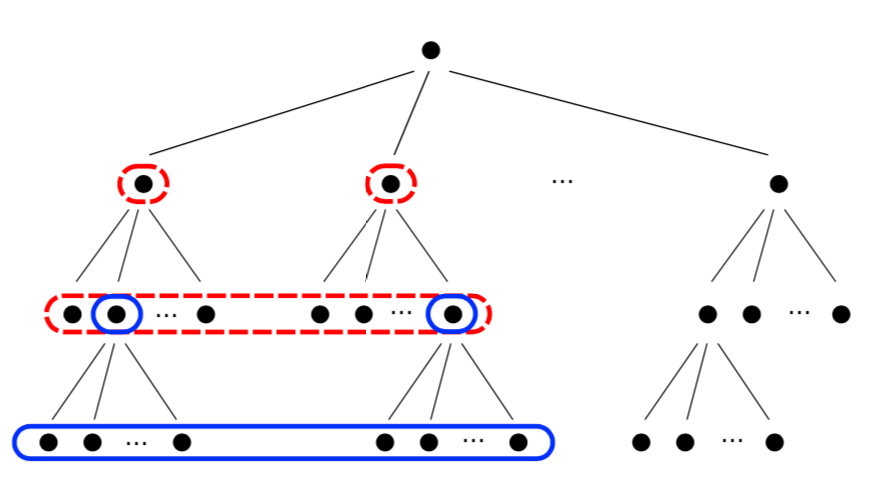
上記のSparse AttentionにおけるAttention Matrixは下図のように図示することができる。
Routing Transformer論文 Figure$\, 1$ $(a)$と$(b)$は前節 で取り扱ったPosition-based Sparse Attentionの計算を自己回帰的(auto regressive)に表したものである。同様に$(c)$がRouting Transformerで用いるRouting Attentionに対応する。
$(c)$の理解にあたっては、まず図では「赤・青・緑」の三色に$3$つのクラスタを対応させたと解釈すると良い。ここで「緑」の行に注目すると、$(5,2)$成分が薄い緑で表されていることが確認できる。この$(5,2)$成分は同じクラスタの位置の隠れ層を参照することに対応する。同様に下からの$2$行は緑であるが、どちらも$2$列目と$5$列目が薄い緑で表されており、$2$番目と$5$番目の隠れ層を参照してそれぞれ計算を行うことも確認できる。
このようにRouting TransformerにおけるRouting Attentionではそれぞれの隠れ層を$k$個のクラスタに分類し、その分類結果に基づいてSparseなAttention Matrixの生成を行う。
Centroid vectorsの計算
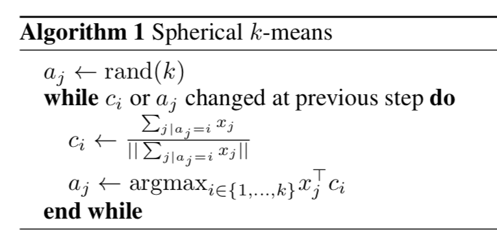
前項 で確認を行ったRouting Attentionはクラスタリングの結果に基づいてSparse Attentionの計算を行う手法である。当項ではクラスタリングに用いるCentroid vectorsの$\boldsymbol{\mu} = (\mu_{1}, \cdots , \mu_{k})$の計算について確認する。
$\boldsymbol{\mu} = (\mu_{1}, \cdots , \mu_{k})$はTransformerの隠れ層の次元である$d$次元の$k$個のベクトルに対応するので、下記のような行列で表すこともできる。
上記の$\boldsymbol{\mu}$は下記のような式に基づいて都度計算を行う。
要確認:上記の計算では$\displaystyle \sum_{i: \mu(Q_i) = l} Q_{i}$のように和を計算する一方で、本来は平均を計算すべきではないか。
まとめ 参考 ・Transformer論文:Attention is All you need[2017] ・A Survey of Transformer ・Star-Transformer ・Longformer ・ETC: Extended Transformer Construction ・Big Bird ・Reformer ・Routing Transformer