
最適化問題を解く際に勾配法などがよく用いられますが、多次元空間上における勾配法などを用いる際には取り得る範囲内でどのステップ幅が良いかを検討する場合があります。この際によく用いられるのが直線探索(line search)です。当記事では直線探索の流れとPythonを用いた計算例をまとめました。
・用語/公式解説
https://www.hello-statisticians.com/explain-terms
Contents
直線探索の概要
目的関数と勾配降下法
目的関数$f(\mathbf{x}_{k})$の$p$次元ベクトル$\mathbf{x}_{k}$に関する勾配降下法(Gradient Descent Method)の漸化式は下記のように表される。
$$
\large
\begin{align}
\mathbf{x}_{k+1} &= \mathbf{x}_{k} – \alpha_{k} \nabla f(\mathbf{x}_{k}) \quad (1) \\
\mathbf{x}_{k} & \in \mathbb{R}^{p} \\
\nabla &= \left(\begin{array}{c} \displaystyle \frac{\partial}{\partial x_1} \\ \vdots \\ \displaystyle \frac{\partial}{\partial x_p} \end{array} \right)
\end{align}
$$
直線探索
前項の「目的関数と勾配降下法」の$(1)$式における$\alpha_{k}$には定数や減衰などを表す関数などを用いることが多いが、多変数関数などを取り扱う際の伝統的な手法の直線探索(line search)も問題によっては役立つ。
直線探索は勾配ベクトルが得られた際に、勾配の方向の目的関数$f(\mathbf{x}_{k})$の値を計算し、最適な値を持つ点のステップ幅を選択するという手法である。原理自体はシンプルである一方でプログラムはやや複雑になるので、次節ではPythonを用いた直線探索の計算例を取り扱った。
直線探索の実装方針
直線探索を実装するにあたっては、探索範囲を元に$\alpha_{k}$の取りうる値を配列で作成し、どの値を用いた際に目的関数が最適値を取るかを調べればよい。たとえば目的関数$f(x)=x^2$の最小化にあたって、$x_k=-2$の際を仮定する。
このとき、$f'(x)=2x$であるので、勾配降下法の式は下記のように表される。
$$
\large
\begin{align}
x_{k+1} &= x_{k} – \alpha_{k} f'(x_k) \\
&= -2 + 4 \alpha_{k}
\end{align}
$$
上記に対し下記を実行することで、$0$〜$1$の$0.01$刻みで$\alpha_{k}$を生成し、どの値が目的関数$f(x)=x^2$を最大化するか調べることができる。
import numpy as np

alpha = np.arange(0,1.01,0.01)
x = -2 + 4*alpha
f_x = x_new**2

x_new = x[np.argmin(f_x)]
print("x_new: {:.1f}".format(x_new))
・実行結果
x_new: 0.0上記では$0.01$刻みで生成した$\alpha_{k}$に対し、取りうる$x_{k+1}$を計算し、$f(x)$を最小にするインデックスをnp.argminを用いて取得した。最小値における詳細は下記を出力することで確認できる。
print(np.argmin(f_x))
print(alpha[np.argmin(f_x)])
print(f_x[np.argmin(f_x)])
・実行結果
50
0.5
0.0
Pythonを用いた直線探索の計算例
問題設定
$$
\large
\begin{align}
f(\mathbf{x}) &= \mathbf{x}^{\mathrm{T}} A \mathbf{x} \\
A &= \left(\begin{array}{cc} 2 & 1 \\ 1 & 2 \end{array} \right) \\
\mathbf{x} & \in \mathbb{R}^{2}
\end{align}
$$
上記のように目的関数$f(\mathbf{x})$を定義する。このとき、等高線上の点は下記のような計算で得ることができる。
$$
\large
\begin{align}
U \mathbf{x} &= \frac{1}{\sqrt{2}} \left(\begin{array}{cc} 1 & -1 \\ 1 & 1 \end{array} \right) \left(\begin{array}{c} \displaystyle \frac{5}{\sqrt{3}} \cos{\frac{\pi}{3}} \\ \displaystyle 5 \sin{\frac{\pi}{3}} \end{array} \right) \\
&= \frac{5}{2 \sqrt{6}} \left(\begin{array}{cc} 1 & -1 \\ 1 & 1 \end{array} \right) \left(\begin{array}{c} 1 \\ 3 \end{array} \right) \\
&= \frac{5}{\sqrt{6}} \left(\begin{array}{c} -1 \\ 2 \end{array} \right) = \left(\begin{array}{c} -2.041 \cdots \\ 4.082 \cdots \end{array} \right)
\end{align}
$$
上記の点から勾配法と共役勾配法によって最小値の探索を行う。また、下記を実行することで点の描画を行うことができる。
import numpy as np
import matplotlib.pyplot as plt

theta = np.linspace(0, 2*np.pi, 100)
c = np.arange(1,6)

x = np.zeros([2,len(theta)])
U = np.array([[1,-1],[1,1]])/np.sqrt(2)
ratio = 1/np.sqrt(3)

plt.figure(figsize=(5,5))
for i in range(len(c)):
    x[0,:] = c[i] * ratio * np.cos(theta)
    x[1,:] = c[i] * np.sin(theta)
    y = np.dot(U,x)
    plt.plot(y[0,:], y[1,:], "g--")

init_pos = np.array([5*ratio*np.cos(np.pi/6), 5*np.sin(np.pi/6)])
init_rotated = np.dot(U,init_pos)

plt.plot([init_rotated[0]],[init_rotated[1]],"ro")

plt.xlim([-5, 5])
plt.ylim([-5, 5])

plt.show()
・実行結果
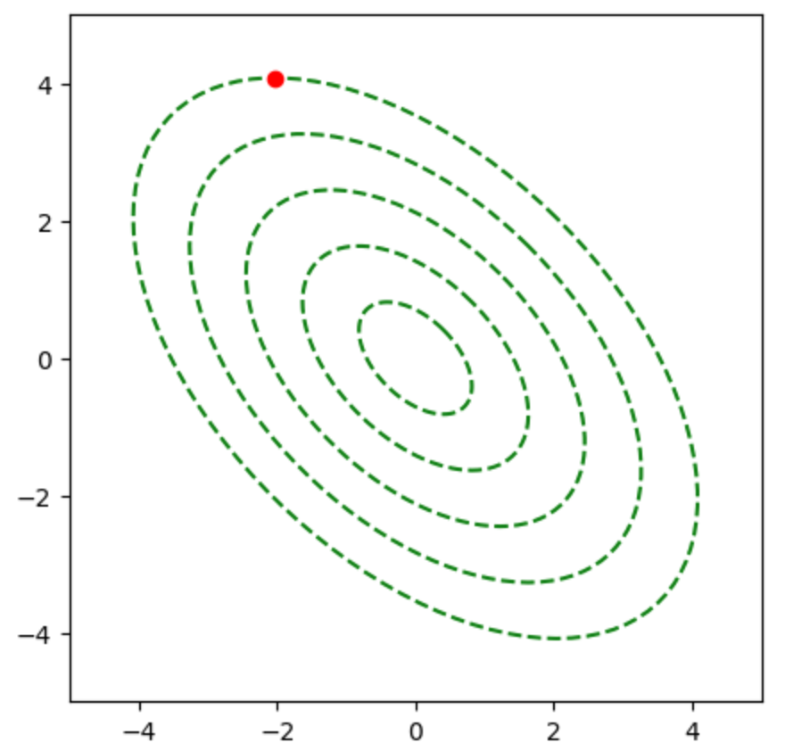
当節では下記の事例を改変し、作成を行なった。
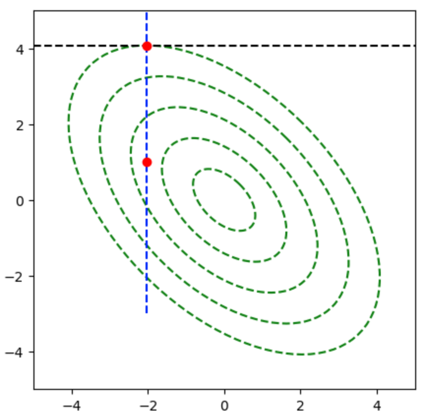
勾配法と直線探索を用いた計算例
下記を実行することで直線探索を行うことができる。
A = np.array([[2, 1], [1, 2]])
U = np.array([[1,-1],[1,1]])/np.sqrt(2)
ratio = 1/np.sqrt(3)

plt.figure(figsize=(5,5))
for i in range(len(c)):
    x = np.zeros([2,len(theta)])
    x[0,:] = c[i] * ratio * np.cos(theta)
    x[1,:] = c[i] * np.sin(theta)
    y = np.dot(U,x)
    plt.plot(y[0,:], y[1,:], "g--")

init_pos = np.array([5*ratio*np.cos(np.pi/3), 5*np.sin(np.pi/3)])
init_rotated = np.dot(U,init_pos)
alpha = np.arange(-5.0,5.01,0.01)

tangent_l = np.dot(U,np.array([init_pos[0]+alpha, init_pos[1]-alpha*np.sqrt(3)/np.tan(np.pi/3)]))
grad = np.dot(U,np.array([init_pos[0]+alpha, init_pos[1]+alpha*np.tan(np.pi/3)/np.sqrt(3)]))

f_x = np.zeros(len(alpha))
for i in range(len(alpha)):
    f_x[i] = np.dot(grad[:,i],np.dot(A,grad[:,i]))
idx = np.argmin(f_x)
x_new = grad[:,idx]

plt.plot(tangent_l[0,:], tangent_l[1,:], "k--")
plt.plot(grad[0,:], grad[1,:], "b--")

plt.plot([init_rotated[0]],[init_rotated[1]],"ro")
plt.plot([x_new[0]],[x_new[1]],"ro")

plt.xlim([-5, 5])
plt.ylim([-5, 5])

plt.show()
・実行結果
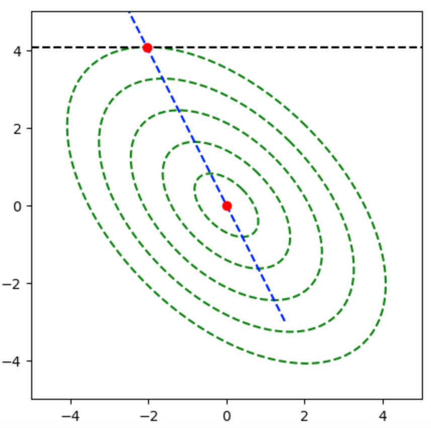
共役勾配法と直線探索を用いた計算例
下記を実行することで共役勾配法における直線探索を行うことができる。
A = np.array([[2,1],[1,2]])
U = np.array([[1,-1],[1,1]])/np.sqrt(2)

x = np.zeros([2,len(theta)])
ratio = 1/np.sqrt(3)

plt.figure(figsize=(5,5))
for i in range(len(c)):
    x[0,:] = c[i] * ratio * np.cos(theta)
    x[1,:] = c[i] * np.sin(theta)
    y = np.dot(U,x)
    plt.plot(y[0,:], y[1,:], "g--")

init_pos = np.array([5*ratio*np.cos(np.pi/3), 5*np.sin(np.pi/3)])
init_rotated = np.dot(U,init_pos)
alpha = np.arange(-5.0,5.01,0.01)

tangent_l = np.dot(U,np.array([init_pos[0]+alpha, init_pos[1]-alpha*np.sqrt(3)/np.tan(np.pi/3)]))
tan, grad = np.dot(U,np.array([1, -np.sqrt(3)/np.tan(np.pi/3)])), np.dot(U,np.array([1, np.tan(np.pi/3)/np.sqrt(3)]))
conjugate_grad = grad - np.dot(tan,np.dot(A,grad))/np.dot(tan,np.dot(A,tan))*tan
conjugate_grad_x = init_rotated[0] + alpha*conjugate_grad[0]
conjugate_grad_y = init_rotated[1] + alpha*conjugate_grad[1]

f_x = np.zeros(len(alpha))
for i in range(len(alpha)):
    f_x[i] = 2*(conjugate_grad_x[i]**2 + conjugate_grad_x[i]*conjugate_grad_y[i] + conjugate_grad_y[i]**2)
idx = np.argmin(f_x)
x_new = np.array([conjugate_grad_x[idx],conjugate_grad_y[idx]])

plt.plot(tangent_l[0,:], tangent_l[1,:], "k--")
plt.plot(conjugate_grad_x, conjugate_grad_y, "b--")

plt.plot([init_rotated[0]],[init_rotated[1]],"ro")
plt.plot([x_new[0]],[x_new[1]],"ro")


plt.xlim([-5, 5])
plt.ylim([-5, 5])

plt.show()
・実行結果
[…] 直線探索(line search)の概要とPythonを用いた計算例 […]