
カルシュ・キューン・タッカー(KKT; Karush Kuhn Tucker)条件は制約付き問題の最適化の際に用いられる$1$次の必要条件で、様々な問題の最適化にあたって用いられます。当記事ではKKT条件など、制約付き問題の最適化における重要なトピックについて取りまとめを行いました。
「新版 数理計画入門(朝倉書店)」の$4.7$節の「制約付き問題の最適性条件」などの内容を参考に作成を行いました。
・用語/公式解説
https://www.hello-statisticians.com/explain-terms
Contents
制約付き問題とKKT条件
問題設定
目的関数$f(\mathbf{x})$の制約付き最適化は下記のように表すことができる。
$$
\large
\begin{align}
\mathrm{Objective} : \quad & f(\mathbf{x}) \, \rightarrow \, \mathrm{Minimize} \\
\mathrm{Constraint} : \quad & c_i(\mathbf{x}) = 0 \quad (i=1, 2, \cdots ,l) \\
& c_i(\mathbf{x}) \leq 0 \quad (i=l+1, l+2, \cdots ,m)
\end{align}
$$
上記は一般的な表記である一方で抽象的なので、以下では下記の具体例を元に確認を行う。
$$
\large
\begin{align}
\mathrm{Objective} : \quad & f(\mathbf{x}) = (x_1-1)^{2} + (x_2-2)^2 \, \rightarrow \, \mathrm{Minimize} \\
\mathrm{Constraint} : \quad & c_1(\mathbf{x}) = x_1^2+x_2^2-2 \leq 0 \\
& c_2(\mathbf{x}) = -x_1+x_2 \leq 0 \\
& c_3(\mathbf{x}) = -x_2 \leq 0
\end{align}
$$
図に基づく最適解の導出と有効制約
最適解の導出にあたってまず制約条件の$c_1(\mathbf{x})$〜$c_3(\mathbf{x})$の取る領域の図示を行う。$x_1^2+x_2^2 \leq 2, x_2 \leq x_1, x_2 \geq 0$が成立する領域は下記を実行することで図示できる。
import numpy as np
import matplotlib.pyplot as plt

r = np.sqrt(2)
theta = np.linspace(0,2*np.pi,100)

x = np.arange(-2., 2.01, 0.01)
x_r1 = np.linspace(0., 1., 100)
x_r2 = np.linspace(1., np.sqrt(2), 100)

plt.plot(r*np.cos(theta), r*np.sin(theta), "g--")
plt.plot(x, 0*x, "g--")
plt.plot(x, x, "g--")

plt.fill_between(x_r1, x_r1*0, x_r1, color="green")
plt.fill_between(x_r2, x_r2*0, np.sqrt(2-x_r2**2+0.0001), color="green")
plt.show()
・実行結果
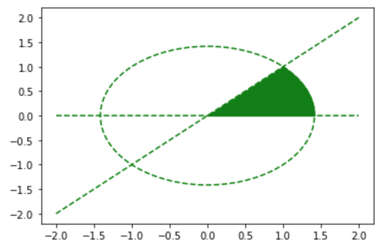
$\sqrt{2-x_1^2}$の値が計算誤差により負の値になる場合があるのでnp.sqrt(2-x_r2**2+0.0001)のように0.0001を加算を行なった。さらに下記を実行することで制約条件の領域に目的関数$f(\mathbf{x}) = (x_1-1)^{2} + (x_2-2)^2$を描画できる。
import numpy as np
import matplotlib.pyplot as plt

r = np.sqrt(2)
theta = np.linspace(0,2*np.pi,100)

x_r1 = np.linspace(0., 1., 100)
x_r2 = np.linspace(1., np.sqrt(2), 100)

x_, y_ = np.arange(-2., 2.01, 0.01), np.arange(-1., 3.01, 0.01)
x, y = np.meshgrid(x_,y_)
z = (x-1)**2 + (y-2)**2

levs = np.arange(0.5,3.5,0.5)**2

plt.plot(r*np.cos(theta), r*np.sin(theta), "k--")

plt.fill_between(x_r1, x_r1*0, x_r1, color="green")
plt.fill_between(x_r2, x_r2*0, np.sqrt(2-x_r2**2+0.0001), color="green")
plt.contour(x,y,z,levels=levs,cmap="viridis")

plt.show()
・実行結果
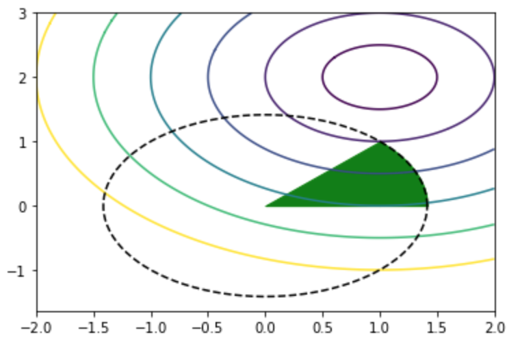
上図の緑の領域の中で目的関数の等高線が中心の紫に近い$(x_1,x_2)=(1,1)$が最適解である。また、最適解の$(1,1)$で等号が成立する制約条件を有効制約というが、この例では$c_1(\mathbf{x}) = x_1^2+x_2^2-2 \leq 0$と$c_2(\mathbf{x}) = -x_1+x_2 \leq 0$が対応する。
KKT条件
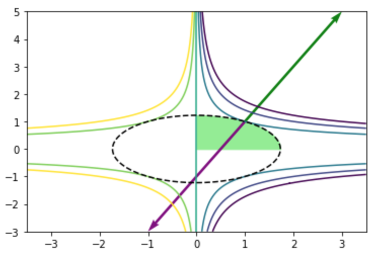
制約付き最適化問題の最適解では基本的に下記で表すように目的関数と有効制約の勾配ベクトルが釣り合うような状態となる。
import numpy as np
import matplotlib.pyplot as plt

r = np.sqrt(2)
theta = np.linspace(0,2*np.pi,100)

x_r1 = np.linspace(0., 1., 100)
x_r2 = np.linspace(1., np.sqrt(2), 100)

x_, y_ = np.arange(-2., 2.01, 0.01), np.arange(-1., 3.01, 0.01)
x, y = np.meshgrid(x_,y_)
z = (x-1)**2 + (y-2)**2

levs = np.arange(0.5,3.5,0.5)**2

plt.plot(r*np.cos(theta), r*np.sin(theta), "k--")

plt.fill_between(x_r1, x_r1*0, x_r1, color="green")
plt.fill_between(x_r2, x_r2*0, np.sqrt(2-x_r2**2+0.0001), color="green")
plt.contour(x,y,z,levels=levs,cmap="viridis")

plt.quiver(1, 1, -1, 1, color="green", angles='xy', scale_units='xy', scale=1)
plt.quiver(1, 1, 1, 1, color="green", angles='xy', scale_units='xy', scale=1)
plt.quiver(1, 1, 0, -2, color="purple", angles='xy', scale_units='xy', scale=1)

plt.show()
・実行結果
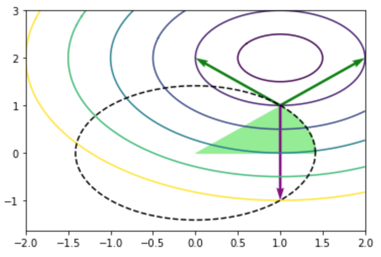
上図では目的関数の勾配ベクトルを紫、有効制約の勾配ベクトルを緑で表した。このような勾配ベクトルの釣り合いを元にカルシュ・キューン・タッカー(KKT; Karush Kuhn Tucker)条件が定式化される。局所最適解$x^{*}$に関してKKT条件は一般的には下記の数式で表される。
$$
\large
\begin{align}
& \nabla f(\mathbf{x}^{*}) + \sum_{i=1}^{n} \lambda_i^{*} \nabla c_i(\mathbf{x}^{*}) = \mathbf{0} \quad (1) \\
& c_i(\mathbf{x}^{*}) = 0 \qquad (i=1, \cdots, l) \\
& c_i(\mathbf{x}^{*}) \leq 0, \lambda_i^{*} \geq 0 \qquad (i=l+1, \cdots, m) \\
& c_i(\mathbf{x}^{*}) < 0, \lambda_i^{*} = 0 \qquad (i=m+1, \cdots, n)
\end{align}
$$
当項で取り扱った図におけるベクトルの釣り合いは上記の$(1)$式に$x_1=1,x_2=1$を代入することで下記のように$\displaystyle \lambda_1=\frac{1}{2}, \lambda_2=1$を得た。
$$
\large
\begin{align}
\nabla f(\mathbf{x}) + \lambda_1 \nabla c_1(\mathbf{x}) + \lambda_2 \nabla c_2(\mathbf{x}) &= \mathbf{0} \\
\nabla [(x_1-1)^2+(x_2-2)^2] + \lambda_1 \nabla (x_1^2+x_2^2-2) + \lambda_2 \nabla (-x_1+x_2) &= \mathbf{0} \\
\left(\begin{array}{c} 2(x_1-1) \\ 2(x_2-2) \end{array} \right) + \lambda_1 \left(\begin{array}{c} 2x_1 \\ 2x_2 \end{array} \right) + \lambda_2 \left(\begin{array}{c} -1 \\ 1 \end{array} \right) &= \left(\begin{array}{c} 0 \\ 0 \end{array} \right) \\
\left(\begin{array}{c} 2(x_1-1) + 2\lambda_1 – \lambda_2 \\ 2(x_2-2) + 2\lambda_1 + \lambda_2 \end{array} \right) &= \left(\begin{array}{c} 0 \\ 0 \end{array} \right) \\
\left(\begin{array}{c} 2 \cdot (1-1) + 2\lambda_1 – \lambda_2 \\ 2 \cdot (1-2) + 2\lambda_1 + \lambda_2 \end{array} \right) &= \left(\begin{array}{c} 0 \\ 0 \end{array} \right) \\
\left(\begin{array}{c} 2\lambda_1 – \lambda_2 \\ 2\lambda_1 + \lambda_2 \end{array} \right) &= \left(\begin{array}{c} 0 \\ 2 \end{array} \right) \\
\lambda_1=\frac{1}{2}, \lambda_2=1 &
\end{align}
$$
当項で取り扱ったKKT条件は制約付き最適化における$1$次の必要条件であり、十分条件ではないことに注意が必要である。十分性については次節で確認を行う。
制約付き問題の最適解の十分条件
凸計画問題とKKT条件
① 目的関数が凸関数
② 等式制約関数$c_i$が$1$次関数
③ 不等式制約関数$c_i$が凸関数
上記が成立する問題を『凸計画問題』というが、凸計画問題でKKT条件が成立する場合の$\mathbf{x}^{*}$はその問題の『大域的最適解』であることが知られている。
ヘッセ行列と$2$次の十分条件
$$
\large
\begin{align}
\mathrm{Objective} : \quad & f(\mathbf{x}) \, \rightarrow \, \mathrm{Minimize} \\
\mathrm{Constraint} : \quad & c_i(\mathbf{x}) = 0 \quad (i=1, 2, \cdots ,l) \\
& c_i(\mathbf{x}) \leq 0 \quad (i=l+1, l+2, \cdots ,m)
\end{align}
$$
上記のように定義した制約付き最適化問題に対し、ラグランジュ関数$L(\mathbf{x},\boldsymbol{\lambda})$を下記のように定義する。
$$
\large
\begin{align}
L(\mathbf{x},\boldsymbol{\lambda}) = f(\mathbf{x}) + \sum_{i=1}^{m} \lambda_{i} c_{i}(\mathbf{x})
\end{align}
$$
上記のラグランジュ関数$L$に対し、変数$\mathbf{x}$に関する勾配ベクトル$\nabla_{x} L(\mathbf{x},\boldsymbol{\lambda})$とヘッセ行列$\nabla_{x}^{2} L(\mathbf{x},\boldsymbol{\lambda})$を下記のように定義する。
$$
\large
\begin{align}
\nabla_{x} L(\mathbf{x},\boldsymbol{\lambda}) &= \nabla f(\mathbf{x}) + \sum_{i=1}^{m} \lambda_{i} \nabla c_{i}(\mathbf{x}) \\
\nabla_{x}^{2} L(\mathbf{x},\boldsymbol{\lambda}) &= \nabla^{2} f(\mathbf{x}) + \sum_{i=1}^{m} \lambda_{i} \nabla^{2} c_{i}(\mathbf{x})
\end{align}
$$
ここで全ての有効制約の勾配ベクトルと直交するベクトルの集合を$M^{*}$とおく。このとき任意のベクトル$\mathbf{y} \in M^{*}$に対して下記が成立することが最適性の$2$次の必要条件である。
$$
\large
\begin{align}
\mathbf{y}^{\mathrm{T}} \nabla_{x}^{2} L(\mathbf{x}^{*},\boldsymbol{\lambda}^{*}) \mathbf{y} \geq 0
\end{align}
$$
同様に任意のベクトル$\mathbf{y} \in M^{*}$に対して下記が成立することが最適性の$2$次の十分条件である。
$$
\large
\begin{align}
\mathbf{y}^{\mathrm{T}} \nabla_{x}^{2} L(\mathbf{x}^{*},\boldsymbol{\lambda}^{*}) \mathbf{y} > 0
\end{align}
$$
$2$次の十分条件の具体例
$$
\large
\begin{align}
\mathrm{Objective} : \quad & f(\mathbf{x}) = -2 x_1 x_2^2 \, \rightarrow \, \mathrm{Minimize} \\
\mathrm{Constraint} : \quad & c_1(\mathbf{x}) = \frac{1}{2} x_1^2 + x_2^2 – \frac{3}{2} \leq 0 \\
& c_2(\mathbf{x}) = -x_1 \leq 0 \\
& c_3(\mathbf{x}) = -x_2 \leq 0
\end{align}
$$
目的関数と制約条件は下記を実行することで図示することができる。
import numpy as np
import matplotlib.pyplot as plt

theta = np.linspace(0,2*np.pi,100)
x_r = np.linspace(0., np.sqrt(3), 100)

x_, y_ = np.arange(-3., 3.01, 0.01), np.arange(-3., 3.01, 0.01)
x, y = np.meshgrid(x_,y_)

z = -2*x*y**2

levs = np.arange(-6,6,2)

plt.plot(np.sqrt(3)*np.cos(theta), np.sqrt(1.5)*np.sin(theta), "k--")
plt.fill_between(x_r, x_r*0, np.sqrt(1.5-0.5*x_r**2), color="green")
plt.contour(x,y,z,levels=levs,cmap="viridis")

plt.colorbar()
plt.show()
・実行結果
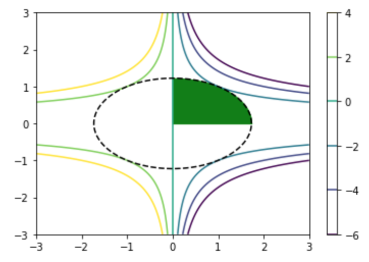
上図より、$x_1=1, x_2=1$のとき目的関数が最小値$f(\mathbf{x}) = -2 \cdot 1 \cdot 1^2 = -2$を取ることや有効制約が$c_1(\mathbf{x})$であることが確認できる。
ここで目的関数$f(\mathbf{x})$の勾配ベクトル$\nabla f(\mathbf{x})$や有効制約$c_1(\mathbf{x})$の勾配ベクトル$\nabla c_1(\mathbf{x})$は下記のように表せる。
$$
\large
\begin{align}
\nabla f(\mathbf{x}) &= \left(\begin{array}{c} -2x_2^2 \\ -4x_1x_2 \end{array} \right) \\
\nabla c_1(\mathbf{x}) &= \left(\begin{array}{c} x_1 \\ 2x_2 \end{array} \right)
\end{align}
$$
上記に$\displaystyle \mathbf{x} = \left(\begin{array}{c} x_1^{*} \\ x_2^{*} \end{array} \right) = \left(\begin{array}{c} 1 \\ 1 \end{array} \right)$を代入すると下記が得られる。
$$
\large
\begin{align}
\nabla f(\mathbf{x}^{*}) &= \left(\begin{array}{c} -2 \\ -4 \end{array} \right) \\
\nabla c_1(\mathbf{x}^{*}) &= \left(\begin{array}{c} 1 \\ 2 \end{array} \right)
\end{align}
$$
上記を元に$\nabla f(\mathbf{x}^{*})$と$\lambda_1 \nabla c_1(\mathbf{x}^{*}) = 2 \nabla c_1(\mathbf{x}^{*})$は下記のように図示できる。
import numpy as np
import matplotlib.pyplot as plt

theta = np.linspace(0,2*np.pi,100)
x_r = np.linspace(0., np.sqrt(3), 100)

x_, y_ = np.arange(-3.5, 3.51, 0.01), np.arange(-3., 5.01, 0.01)
x, y = np.meshgrid(x_,y_)

z = -2*x*y**2

levs = np.arange(-6,6,2)

plt.plot(np.sqrt(3)*np.cos(theta), np.sqrt(1.5)*np.sin(theta), "k--")
plt.fill_between(x_r, x_r*0, np.sqrt(1.5-0.5*x_r**2), color="lightgreen")
plt.contour(x,y,z,levels=levs,cmap="viridis")

plt.quiver(1, 1, -2, -4, color="purple", angles='xy', scale_units='xy', scale=1)
plt.quiver(1, 1, 2, 4, color="green", angles='xy', scale_units='xy', scale=1)

plt.show()
・実行結果
また、ヘッセ行列$\nabla^{2} f(\mathbf{x})$と$\nabla^{2} c_1(\mathbf{x})$は下記のように得られる。
$$
\large
\begin{align}
\nabla^{2} f(\mathbf{x}) &= \left(\begin{array}{cc} 0 & -4x_2 \\ -4x_2 & -4x_1 \end{array} \right) \\
\nabla^{2} c_1(\mathbf{x}) &= \left(\begin{array}{cc} 1 & 0 \\ 0 & 2 \end{array} \right)
\end{align}
$$
上記より$\mathbf{x}^{*}$におけるラグランジュ関数のヘッセ行列$\nabla_{x}^{2} L(\mathbf{x}^{*},\boldsymbol{\lambda}^{*})$は下記のように得られる。
$$ \large \begin{align} \nabla_{x}^{2} L(\mathbf{x}^{*},\boldsymbol{\lambda}^{*}) &= \nabla^{2} f(\mathbf{x}^{*}) + \lambda_{1}^{*} \nabla^{2} c_1(\mathbf{x}^{*}) \\
&= \left(\begin{array}{cc} 0 & -4 \cdot 1 \\ -4 \cdot 1 & -4 \cdot 1 \end{array} \right) + 2 \left(\begin{array}{cc} 1 & 0 \\ 0 & 2 \end{array} \right) \\
&= \left(\begin{array}{cc} 2 & -4 \\ -4 & 0 \end{array} \right)
\end{align}
$$
ここで最適解$\mathbf{x}^{*}$における有効制約の勾配ベクトル$\displaystyle \nabla c_1(\mathbf{x}^{*}) = \left(\begin{array}{c} 1 \\ 2 \end{array} \right)$に垂直なベクトル$\mathbf{y}$は下記のように表せる。
$$
\large
\begin{align}
\mathbf{y} = \left(\begin{array}{c} 2t \\ -t \end{array} \right), \quad t \in \mathbb{R} \quad \mathrm{and} \quad t \neq 0
\end{align}
$$
上記に対し、$\mathbf{y}^{\mathrm{T}} \nabla_{x}^{2} L(\mathbf{x}^{*},\boldsymbol{\lambda}^{*}) \mathbf{y}$は下記のように表せる。
$$
\large
\begin{align}
\mathbf{y}^{\mathrm{T}} \nabla_{x}^{2} L(\mathbf{x}^{*},\boldsymbol{\lambda}^{*}) \mathbf{y} &= \left(\begin{array}{cc} 2t & -t \end{array} \right) \left(\begin{array}{cc} 2 & -4 \\ -4 & 0 \end{array} \right) \left(\begin{array}{c} 2t \\ -t \end{array} \right) \\
&= \left(\begin{array}{cc} 8t & -8t \end{array} \right) \left(\begin{array}{c} 2t \\ -t \end{array} \right) \\
&= 24t^2 > 0
\end{align}
$$
上記より$\mathbf{y}^{\mathrm{T}} \nabla_{x}^{2} L(\mathbf{x}^{*},\boldsymbol{\lambda}^{*}) \mathbf{y} > 0$が成立するので$2$次の十分条件が成立することが確認できる。