
共役勾配法(Conjugate Gradient Method)は等高線が同心楕円で表される場合の最適化にあたって有用な手法です。当記事では具体的な二次形式に対して共役勾配法を元に最適化を行う流れをPythonを用いて計算やグラフの描画を行いました。
当記事は「共役勾配法:日本オペレーション・リサーチ学会 $1987$年$6$月号」などを参考に作成を行いました。
https://orsj.org/wp-content/or-archives50/pdf/bul/Vol.32_06_363.pdf
・用語/公式解説
https://www.hello-statisticians.com/explain-terms
二次形式の等高線のグラフ化
二次形式の式定義
$$
\large
\begin{align}
f(\mathbf{x}) &= \mathbf{x}^{\mathrm{T}} A \mathbf{x} \quad (1) \\
A &= \left(\begin{array}{cc} 2 & 1 \\ 1 & 2 \end{array} \right) \\
\mathbf{x} &= \left(\begin{array}{c} x_1 \\ x_2 \end{array} \right)
\end{align}
$$
$(1)$式のように定義された二次形式$f(\mathbf{x}) = \mathbf{x}^{\mathrm{T}} A \mathbf{x}$の最小点を以下、共役勾配法を用いて計算を行う。
二次形式の図形的解釈
行列$A$の固有値と長さ$1$の固有ベクトルを$\lambda_{1}, \lambda_{2}$、$\mathbf{e}_{1}, \mathbf{e}_{2}$とおくと、それぞれ下記のように得られる。
$$
\large
\begin{align}
\lambda_{1} &= 3, \, \mathbf{e}_{1} = \frac{1}{\sqrt{2}} \left(\begin{array}{c} 1 \\ 1 \end{array} \right) \\
\lambda_{2} &= 1, \, \mathbf{e}_{2} = \frac{1}{\sqrt{2}} \left(\begin{array}{c} -1 \\ 1 \end{array} \right)
\end{align}
$$
上記が正しいことは$A \mathbf{e}_{i} = \lambda_{i} \mathbf{e}_{i}$が成立することから確認できる。ここで任意のベクトル$\mathbf{x}$を係数$a_1, a_2$を用いて下記のように表すことができる。
$$
\large
\begin{align}
\mathbf{x} = a_1 \mathbf{e}_{1} + a_2 \mathbf{e}_{2} \quad (2)
\end{align}
$$
このとき$(1)$式に$(2)$式を代入すると下記が得られる。
$$
\large
\begin{align}
f(\mathbf{x}) &= \mathbf{x}^{\mathrm{T}} A \mathbf{x} \\
&= (a_1 \mathbf{e}_{1} + a_2 \mathbf{e}_{2})^{\mathrm{T}} A (a_1 \mathbf{e}_{1} + a_2 \mathbf{e}_{2}) \\
&= (a_1 \mathbf{e}_{1} + a_2 \mathbf{e}_{2})^{\mathrm{T}} (\lambda_1 a_1 \mathbf{e}_{1} + \lambda_2 a_2 \mathbf{e}_{2}) \\
&= \lambda_{1} a_{1}^{2} + \lambda_{2} a_{2}^{2} \\
&= 3 a_{1}^{2} + a_{2}^{2} \quad (3)
\end{align}
$$
上記の計算にあたっては$\mathbf{e}_{i}^{\mathrm{T}} \mathbf{e}_{i}=1, \mathbf{e}_{1}^{\mathrm{T}} \mathbf{e}_{2}=0$が成立することを用いた。ここで$f(\mathbf{x})=C$の等高線は$(3)$式より下記のように得られる。
$$
\large
\begin{align}
f(\mathbf{x}) = 3 a_{1}^{2} + a_{2}^{2} &= C \\
\frac{a_{1}^{2}}{\sqrt{C/3}^{2}} + \frac{a_{2}^{2}}{\sqrt{C}^{2}} &= 0 \quad (4)
\end{align}
$$
上記は楕円の方程式に一致する。ここで$(2)$式より、$a_1, a_2$は基底$\mathbf{e}_{1}, \mathbf{e}_{2}$に対応するが、$\mathbf{e}_{1}, \mathbf{e}_{2}$は$\displaystyle \left(\begin{array}{c} 1 \\ 0 \end{array} \right), \, \left(\begin{array}{c} 0 \\ 1 \end{array} \right)$をそれぞれ$\displaystyle \frac{\pi}{4}$回転させたベクトルに一致する。
よって、$(4)$式に基づいて楕円を描き、原点を中心に$\displaystyle \frac{\pi}{4}$回転させることで楕円の等高線の描画を行うことができる。次項でPythonを用いたグラフ化について取り扱った。
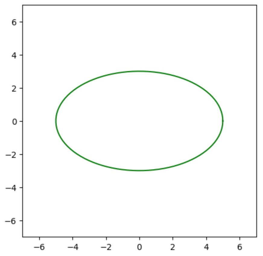
楕円の描画
$$
\large
\begin{align}
\frac{x^2}{5^2} + \frac{y^2}{3^2} = 1 \quad (5)
\end{align}
$$
上記の$(5)$式のような楕円の方程式が得られた際に等高線の描画を行うにあたっては媒介変数表示を用いればよい。具体的には$x = 5 \cos{\theta}, \, y = 3 \sin{\theta}$が下記のように$(5)$について成立することを活用する。
$$
\large
\begin{align}
\frac{x^2}{5^2} + \frac{y^2}{3^2} &= \frac{\cancel{5^2} \cos^{2}{\theta}}{\cancel{5^2}} + \frac{\cancel{3^2} \sin^{2}{\theta}}{\cancel{3^2}} \\
&= \cos^{2}{\theta} + \sin^{2}{\theta} = 1
\end{align}
$$
ここまでの内容を元に、$(5)$式は下記を実行することで描画できる。
import numpy as np
import matplotlib.pyplot as plt

theta = np.linspace(0, 2*np.pi, 100)

x = 5 * np.cos(theta)
y = 3 * np.sin(theta)

plt.figure(figsize=(5,5))
plt.plot(x, y, "g-")

plt.xlim([-7, 7])
plt.ylim([-7, 7])

plt.show()
・実行結果
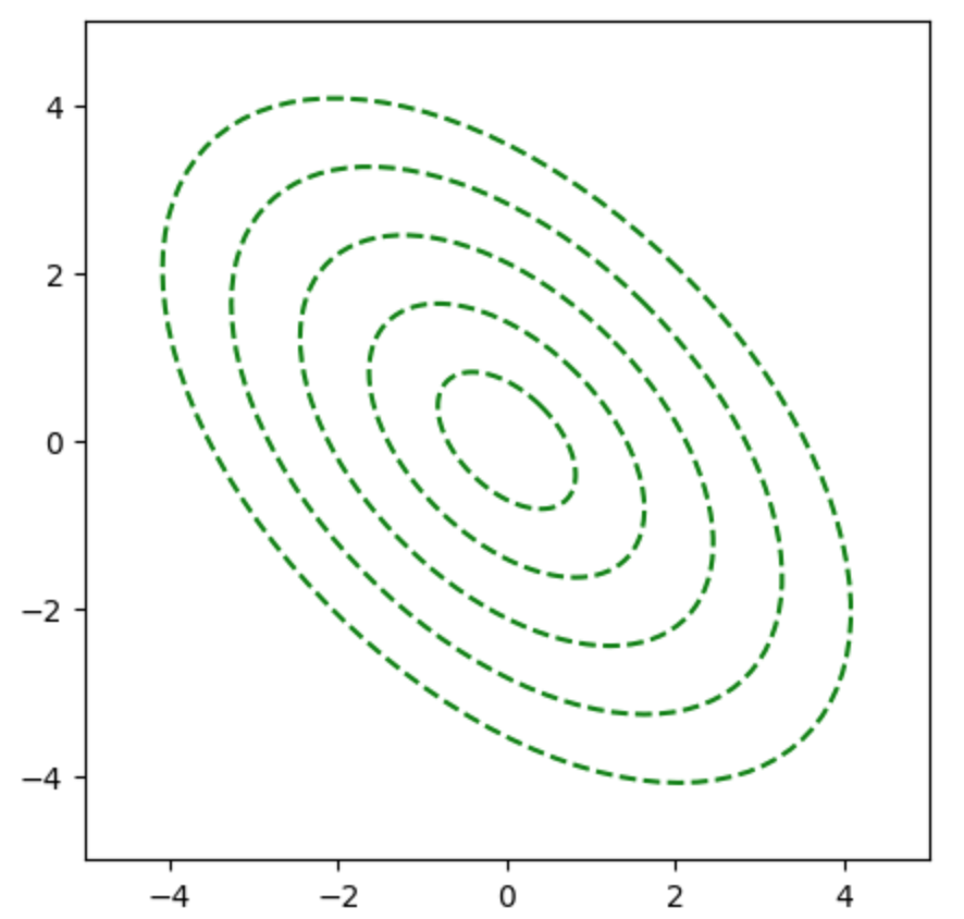
上記の描画に回転を組み合わせることで$(4)$式が描画できる。$C=1,2,3,4,5$について、下記を実行することで同心楕円を描くことができる。
theta = np.linspace(0, 2*np.pi, 100)
c = np.arange(1,6)

x = np.zeros([2,len(theta)])
U = np.array([[1,-1],[1,1]])/np.sqrt(2)
ratio = 1/np.sqrt(3)

plt.figure(figsize=(5,5))
for i in range(len(c)):
    x[0,:] = c[i] * ratio * np.cos(theta)
    x[1,:] = c[i] * np.sin(theta)
    y = np.dot(U,x)
    plt.plot(y[0,:], y[1,:], "g--")

plt.xlim([-5, 5])
plt.ylim([-5, 5])

plt.show()
・実行結果
回転行列を用いた計算にあたっては下記で詳しく取り扱った。
共役勾配法の実行
同心楕円の接線と勾配
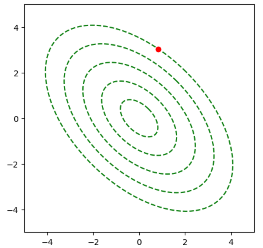
同心楕円上の点は下記のように$\displaystyle \mathbf{x} = \left(\begin{array}{c} \displaystyle \sqrt{\frac{C}{3}} \cos{\theta} \\ \sqrt{C} \sin{\theta} \end{array} \right)$を原点を中心に$\displaystyle \frac{\pi}{4}$回転させることで得られる。
$$
\large
\begin{align}
R \left( \frac{\pi}{4} \right) \mathbf{x} = \left(\begin{array}{cc} 1 & -1 \\ 1 & 1 \end{array} \right) \frac{1}{\sqrt{2}} \left(\begin{array}{c} \displaystyle \sqrt{\frac{C}{3}} \cos{\theta} \\ \sqrt{C} \sin{\theta} \end{array} \right)
\end{align}
$$
上記の式に基づいて、同心楕円上の点は下記を実行することで得ることができる。
x = np.zeros([2,len(theta)])
U = np.array([[1,-1],[1,1]])/np.sqrt(2)
ratio = 1/np.sqrt(3)

plt.figure(figsize=(5,5))
for i in range(len(c)):
    x[0,:] = c[i] * ratio * np.cos(theta)
    x[1,:] = c[i] * np.sin(theta)
    y = np.dot(U,x)
    plt.plot(y[0,:], y[1,:], "g--")

init_pos = np.dot(U,x[:,5])

plt.plot([init_pos[0]],[init_pos[1]],"ro")

plt.xlim([-5, 5])
plt.ylim([-5, 5])

plt.show()
・実行結果
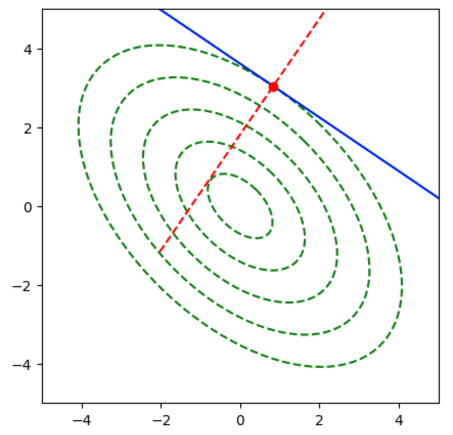
また、$\displaystyle \left(\begin{array}{c} \displaystyle \sqrt{\frac{C}{3}} \cos{\theta} \\ \sqrt{C} \sin{\theta} \end{array} \right)$における接線に平行なベクトルを$\mathbf{v}_{1}$、$\mathbf{v}_{1}$の傾きを$\Delta_{1}$、法線ベクトルを$\mathbf{v}_{2}$とおくと、$\Delta_{1}$は下記のように表すことができる。
$$
\large
\begin{align}
\Delta_{1} &= \frac{dx_2}{dx_1} = \frac{\displaystyle \frac{dx_2}{d\theta}}{\displaystyle \frac{dx_1}{d\theta}} \\
&= \frac{\displaystyle \sqrt{C} \cos{\theta}}{\displaystyle -\sqrt{\frac{C}{3}} \sin{\theta}} \\
&= -\frac{\sqrt{3}}{\tan{\theta}}
\end{align}
$$
ここで$\mathbf{v}_{1} \perp \mathbf{v}_{2}$より$\mathbf{v}_{1} \cdot \mathbf{v}_{2}=0$であるので、$\mathbf{v}_{1}$と$\mathbf{v}_{2}$は下記のように得られる。
$$
\large
\begin{align}
\mathbf{v}_{1} &= \left(\begin{array}{c} 1 \\ \displaystyle -\frac{\sqrt{3}}{\tan{\theta}} \end{array} \right) \quad (6) \\
\mathbf{v}_{2} &= \left(\begin{array}{c} 1 \\ \displaystyle \frac{\tan{\theta}}{\sqrt{3}} \end{array} \right) \quad (7)
\end{align}
$$
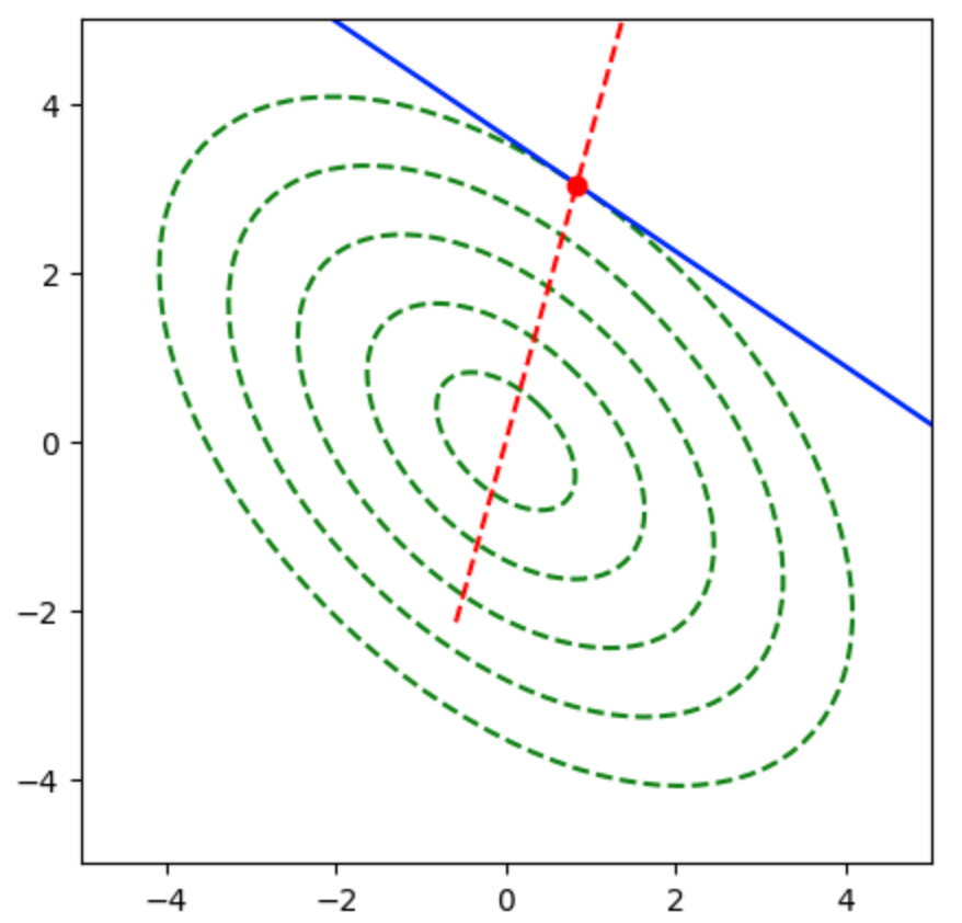
$(6),(7)$式に基づいて接線と法線は下記のように図示できる。
x = np.zeros([2,len(theta)])
U = np.array([[1,-1],[1,1]])/np.sqrt(2)
ratio = 1/np.sqrt(3)

plt.figure(figsize=(5,5))
for i in range(len(c)):
    x[0,:] = c[i] * ratio * np.cos(theta)
    x[1,:] = c[i] * np.sin(theta)
    y = np.dot(U,x)
    plt.plot(y[0,:], y[1,:], "g--")

init_pos = np.dot(U,x[:,5])
alpha = np.arange(-5.0,5.01,0.01)

tangent_l = np.dot(U,np.array([x[0,5]+alpha, x[1,5]-alpha*np.sqrt(3)/np.tan(theta[5])]))
grad = np.dot(U,np.array([x[0,5]+alpha, x[1,5]+alpha*np.tan(theta[5])/np.sqrt(3)]))

plt.plot(tangent_l[0,:], tangent_l[1,:], "b-")
plt.plot(grad[0,:], grad[1,:], "r--")
plt.plot([init_pos[0]],[init_pos[1]],"ro")

plt.xlim([-5, 5])
plt.ylim([-5, 5])

plt.show()
・実行結果
共役勾配法
$\mathbf{d}_{1}=\mathbf{v}_{1}$とおくとき、対称行列$A$について$\mathbf{d}_{1}$と共役であるベクトル$\mathbf{d}_{2}$は、下記の式に基づいて得られる。
$$
\large
\begin{align}
\mathbf{d}_{2} = \mathbf{v}_{2} – \frac{\mathbf{v}_{1}^{\mathrm{T}} A \mathbf{v}_{2}}{\mathbf{v}_{1}^{\mathrm{T}} A \mathbf{v}_{1}} \mathbf{v}_{1} \quad (8)
\end{align}
$$
共役勾配法の式に関しては下記で詳しく取り扱った。
$(8)$式に基づいて下記のような計算を行うことで、$\mathbf{d}_{2}$の描画を行うことができる。
A = np.array([[2,1],[1,2]])
U = np.array([[1,-1],[1,1]])/np.sqrt(2)

x = np.zeros([2,len(theta)])
ratio = 1/np.sqrt(3)

plt.figure(figsize=(5,5))
for i in range(len(c)):
    x[0,:] = c[i] * ratio * np.cos(theta)
    x[1,:] = c[i] * np.sin(theta)
    y = np.dot(U,x)
    plt.plot(y[0,:], y[1,:], "g--")

init_pos = np.dot(U,x[:,5])
alpha = np.arange(-5.0,5.01,0.01)

tangent_l = np.dot(U,np.array([x[0,5]+alpha, x[1,5]-alpha*np.sqrt(3)/np.tan(theta[5])]))
tan, grad = np.dot(U,np.array([1, -np.sqrt(3)/np.tan(theta[5])])), np.dot(U,np.array([1, np.tan(theta[5])/np.sqrt(3)]))
conjugate_grad = grad - np.dot(tan,np.dot(A,grad))/np.dot(tan,np.dot(A,tan))*tan
conjugate_grad_x = init_pos[0] + alpha*conjugate_grad[0]
conjugate_grad_y = init_pos[1] + alpha*conjugate_grad[1]

plt.plot(tangent_l[0,:], tangent_l[1,:], "b-")
plt.plot(conjugate_grad_x, conjugate_grad_y, "r--")
plt.plot([init_pos[0]],[init_pos[1]],"ro")

plt.xlim([-5, 5])
plt.ylim([-5, 5])

plt.show()
・実行結果
プログラムの理解にあたっては、19行目で用いたtanが$\mathbf{v}_{1}$、gradが$\mathbf{v}_{2}$、conjugate_gradが$\mathbf{d}_{2}$に対応することに着目すると良い。また、最小点は$\mathbf{d}_{2}$を元にline searchを行うことで得られる。
[…] 共役勾配法(Conjugate Gradient Method)のPythonを用いた計算例 […]
[…] $(1)$式の詳細は「共役勾配法の原理と具体的な計算例」、「共役勾配法のPythonを用いた計算例」などで取り扱った。ここで$(1)$式の対称行列$A$は数値で与えられることもあるが、多変数関数の最適化などの場合はヘッセ行列$H$が用いられる。 […]
[…] 共役勾配法(Conjugate Gradient Method)のPythonを用いた計算例 […]