ガウス過程の流れとPythonプログラムを用いたガウス過程の作成

カーネル法(Kernel methods)の応用例の一つにガウス過程(Gaussian Process)やガウス過程回帰(Gaussian Process Regression)があるので、当記事ではガウス過程の導出の流れとPythonプログラムを用いたガウス過程の作成に関して取り扱います。

作成にあたっては「ガウス過程と機械学習」の$3$章の「ガウス過程」と「パターン認識と機械学習」の$6.4$節の「Gaussian Processes」を参考にしました。

また、$(\mathrm{o.xx})$の形式の式番号は「パターン認識と機械学習」の式番号に対応させました。

ガウス過程と機械学習 (機械学習プロフェッショナルシリーズ)

持橋大地, 大羽成征

2,310円(04/29 09:24時点)

発売日: 2019/03/09

Amazon

パターン認識と機械学習 下 (ベイズ理論による統計的予測)

C.M. ビショップ

8,580円(04/28 14:38時点)

Amazon

・参考
カーネル関数の計算とPythonを用いたグラフの作成

ガウス過程回帰の仕組み

線形回帰とカーネル法

$N$個のサンプルの$D$次元特徴量ベクトル$\mathbf{x}_{1}, …, \mathbf{x}_{N}$を考える。このとき$\mathbf{x}_{n}$は下記のように表せる。
$$
\large
\begin{align}
\mathbf{x}_{n} = \left( \begin{array}{c} x_{n1} \\ \vdots \\ x_{nD} \end{array} \right)
\end{align}
$$

ここで、$D$次元ベクトル$\mathbf{x}_{n}$に対して$M$次元の基底$\phi_{0}(\mathbf{x}_n),…,\phi_{M-1}(\mathbf{x}_n)$を考える。このときデザイン行列$\boldsymbol{\Phi}$を下記のように定める。
$$
\large
\begin{align}
\boldsymbol{\Phi} = \left( \begin{array}{ccc} \phi_{0}(\mathbf{x}_{1}) & \cdots & \phi_{M-1}(\mathbf{x}_{1}) \\ \vdots & \ddots & \vdots \\ \phi_{0}(\mathbf{x}_{N}) & \cdots & \phi_{M-1}(\mathbf{x}_{N}) \end{array} \right)
\end{align}
$$

このとき、$D$次元ベクトル$\mathbf{x}_{n}$に対して、予測値の$y_{n}$を計算することを考える。$N$個のサンプルの予測値のベクトルを$\mathbf{y}$で定め、$M$次元の重みパラメータ$w_{0},…,w_{M-1}$を用いて下記のように表す。
$$
\large
\begin{align}
\mathbf{y} &= \boldsymbol{\Phi} \mathbf{w} \\
\left( \begin{array}{c} y_{1} \\ \vdots \\ y_{n} \end{array} \right) &= \left( \begin{array}{ccc} \phi_{0}(\mathbf{x}_{1}) & \cdots & \phi_{M-1}(\mathbf{x}_{1}) \\ \vdots & \ddots & \vdots \\ \phi_{0}(\mathbf{x}_{N}) & \cdots & \phi_{M-1}(\mathbf{x}_{N}) \end{array} \right) \left( \begin{array}{c} w_{0} \\ \vdots \\ w_{M-1} \end{array} \right)
\end{align}
$$

以下、$\mathbf{w} \sim \mathcal{N}(0,\lambda^2 I_{M})$であると仮定し、$\mathbf{y}$の分布について考える。$\mathbf{y}$の期待値ベクトル$\mathbb{E}[\mathbf{y}]$と共分散行列$\mathrm{Cov}[\mathbf{y}]$はそれぞれ下記のように計算できる。
$$
\large
\begin{align}
\mathbb{E}[\mathbf{y}] &= \mathbb{E}[\boldsymbol{\Phi} \mathbf{w}] \\
&= \boldsymbol{\Phi} \mathbb{E}[\mathbf{w}] = \mathbf{0} \quad (6.52) \\
\mathrm{Cov}[\mathbf{y}] &= \mathbb{E}[\mathbf{y}\mathbf{y}^{\mathrm{T}}] \\
&= \mathbb{E}[\boldsymbol{\Phi} \mathbf{w}(\boldsymbol{\Phi} \mathbf{w})^{\mathrm{T}}] \\
&= \boldsymbol{\Phi} \mathbb{E}[\mathbf{w}\mathbf{w}^{\mathrm{T}}] \boldsymbol{\Phi}^{\mathrm{T}} \\
&= \boldsymbol{\Phi} \lambda^2 I_{M} \boldsymbol{\Phi}^{\mathrm{T}} \\
&= \lambda^2 \boldsymbol{\Phi} \boldsymbol{\Phi}^{\mathrm{T}} \quad (6.53)’
\end{align}
$$

よって$\mathbf{y} \sim \mathcal{N}(\mathbf{0},\lambda^2 \boldsymbol{\Phi} \boldsymbol{\Phi}^{\mathrm{T}})$が成立する。

カーネル関数の定義

前項の導出結果の$\mathbf{y} \sim \mathcal{N}(\mathbf{0},\lambda^2 \boldsymbol{\Phi} \boldsymbol{\Phi}^{\mathrm{T}})$は下記のように表すこともできる。
$$
\large
\begin{align}
p(\mathbf{y}) = \mathcal{N}(\mathbf{0},\lambda^2 \boldsymbol{\Phi} \boldsymbol{\Phi}^{\mathrm{T}})
\end{align}
$$

ここで上記の$\lambda^2 \boldsymbol{\Phi} \boldsymbol{\Phi}^{\mathrm{T}}$に関して下記のように$K$を定義することを考える。
$$
\large
\begin{align}
K = \lambda^2 \boldsymbol{\Phi} \boldsymbol{\Phi}^{\mathrm{T}}
\end{align}
$$

ここで行列$K$の$i$行$j$列の要素$K_{ij}$はデザイン行列$\boldsymbol{\Phi}$の定義より下記のように表せる。
$$
\large
\begin{align}
K_{ij} &= \lambda^2 \sum_{m=0}^{M-1} \phi_{m}(\mathbf{x}_{i}) \phi_{m}(\mathbf{x}_{j}) \\
&= \lambda^2 \boldsymbol{\phi}(\mathbf{x}_{i})^{\mathrm{T}} \boldsymbol{\phi}(\mathbf{x}_{j}) = k(\mathbf{x}_{i},\mathbf{x}_{j}) \quad (6.54)’ \\
\boldsymbol{\phi}(\mathbf{x}_{i}) &= \left( \begin{array}{c} \phi_{0}(\mathbf{x}_{i}) \\ \vdots \\ \phi_{M-1}(\mathbf{x}_{i}) \end{array} \right)
\end{align}
$$

ここで上記の$k(\mathbf{x}_{i},\mathbf{x}_{j})$はカーネル関数であるが、以下では下記のようにカーネル関数を定めることを考える。
$$
\large
\begin{align}
k(\mathbf{x}_{i},\mathbf{x}_{j}) = \theta_{0} \exp \left[ -\frac{\theta_1}{2}||\mathbf{x}_{i}-\mathbf{x}_{j}||^2 \right] + \theta_2 + \theta_3 \mathbf{x}_{i}^{\mathrm{T}}\mathbf{x}_{j} \quad (6.63)’
\end{align}
$$

ここで上記の第$1$項の$\displaystyle \theta_{0} \exp \left[ -\frac{\theta_1}{2}||\mathbf{x}_{i}-\mathbf{x}_{j}||^2 \right]$は「パターン認識と機械学習」の$(6.23)$式のガウシアンカーネルに基づく。このガウシアンカーネルは無限次元の特徴量ベクトルに基づくカーネル関数であることを「パターン認識と機械学習」の演習$6.11$の解答で示した。また、$(6.13), (6.15), (6.17)$式などを用いて$(6.63)’$式が有効なカーネル関数であることも示せる。よって、$(6.63)’$式は無限次元の特徴量ベクトルに基づくカーネル関数であると考えられる。

このとき、$p(\mathbf{y}) = \mathcal{N}(\mathbf{0},\lambda^2 \boldsymbol{\Phi} \boldsymbol{\Phi}^{\mathrm{T}}) = \mathcal{N}(\mathbf{0},K)$に基づいてガウス過程$\mathbf{y}$の生成を行うことができる。

ガウス過程の生成

前項の流れで計算した$K$を用いて$p(\mathbf{y}) = \mathcal{N}(\mathbf{0},K)$に基づいて$\mathbf{y}$を生成することを以下考える。

上記を考える際に多次元正規分布のサンプルの生成に関して考えれば良いが、共分散行列$K$を行列分解することでサンプルの生成を行うことができる。まず、「ガウス過程と機械学習」で取り扱うcholesky分解を参考に$K = LL^{\mathrm{T}}$のように行列分解できると考える。

この際に$\mathbf{x} \sim \mathcal{N}(\mathbf{0},I_M)$からサンプリングを行なった$\mathbf{x}$に対して$L\mathbf{x}$を計算することで$p(\mathbf{y}) = \mathcal{N}(\mathbf{0},K)$に基づいて$\mathbf{y}$を生成できる。$\mathbf{y}=L\mathbf{x}$に基づいて生成を行なった$\mathbf{y}$に関して$\mathbf{y} \sim \mathcal{N}(\mathbf{0},\mathbf{\Sigma})$が成立することに関する詳しい導出は「パターン認識と機械学習」の演習$11.5$の解答で取り扱った。

Pythonプログラムを用いたガウス過程の作成

カーネル関数の計算

まずはカーネル関数の計算に関して取り扱う。下記を実行することでカーネル関数の計算と可視化を行うことができる。

import numpy as np
import matplotlib.pyplot as plt

theta = np.array([1., 4., 0., 0.])

x = np.arange(-1.,1.01,0.01)
n = x.shape[0]
K = np.zeros([n,n])

for i in range(n):
    for j in range(n):
        K[i,j] = theta[0]*np.exp(-theta[1]*(x[i]-x[j])**2/2) + theta[2] + theta[3]*x[i]*x[j]

plt.imshow(K)
plt.show()

・実行結果

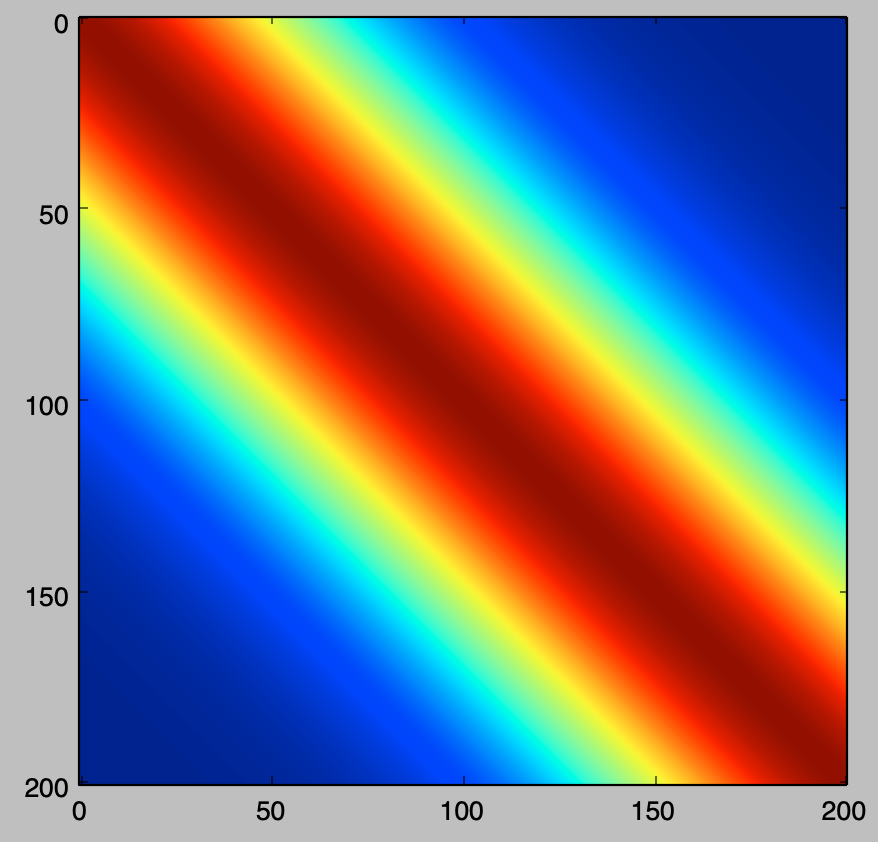
上記より、$x$の値が近い所のカーネル関数が大きい値を持つことが確認できる。

行列分解

cholesky分解

共分散行列のcholesky分解と可視化は下記を実行することで計算できる。

np.random.seed(0)

theta = np.array([1., 10., 0., 0.])

x = np.arange(0.,5.1,0.1)
n = x.shape[0]
K = np.zeros([n,n])

for i in range(n):
    for j in range(n):
        K[i,j] = theta[0]*np.exp(-theta[1]*(x[i]-x[j])**2/2) + theta[2] + theta[3]*x[i]*x[j]

L = np.linalg.cholesky(K)

plt.subplot(121)
plt.imshow(K)

plt.subplot(122)
plt.imshow(L)

plt.show()

・実行結果

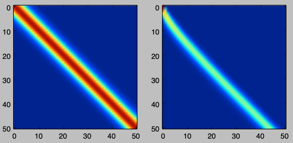
cholesky分解は対称行列を下三角行列に分解する手法であるので、可視化の結果は妥当であると考えることができる。

Eckart-Young分解

cholesky分解は下三角行列への分解であるが、固有値分解の考え方を元に下記のようにEckart-Young分解を行うこともできる。

np.random.seed(0)

theta = np.array([1., 10., 0., 0.])

x = np.arange(0.,10.1,0.1)
n = x.shape[0]
K = np.zeros([n,n])

for i in range(n):
    for j in range(n):
        K[i,j] = theta[0]*np.exp(-theta[1]*(x[i]-x[j])**2/2) + theta[2] + theta[3]*x[i]*x[j]

Lamb, U_T = np.linalg.eig(K)
Lamb, U_T = Lamb.real, U_T.real
U = U_T.T

A = np.dot(U_T,np.diag(np.sqrt(Lamb)))

plt.subplot(121)
plt.imshow(K)

plt.subplot(122)
plt.imshow(A)

plt.show()

・実行結果

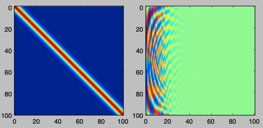
分解後の行列の左側の要素が値を持ち、右側が値を持たないのは固有値の大きいものからベクトルを並べたことに起因する。

ガウス過程の生成

import numpy as np
import matplotlib.pyplot as plt
from scipy import stats

np.random.seed(0)

theta = np.array([1., 10., 0., 0.])

x = np.arange(0.,2.02,0.02)
n = x.shape[0]
K = np.zeros([n,n])

for i in range(n):
    for j in range(n):
        K[i,j] = theta[0]*np.exp(-theta[1]*(x[i]-x[j])**2/2) + theta[2] + theta[3]*x[i]*x[j]

Lamb, U_T = np.linalg.eig(K)
Lamb, U_T = Lamb.real, U_T.real
U = U_T.T

A = np.dot(U_T,np.diag(np.sqrt(Lamb+10**(-12.))))

for i in range(5):
    y = np.dot(A,stats.norm.rvs(loc=0,scale=1,size=n))
    plt.plot(x,y)

plt.show()

・実行結果

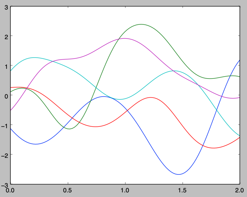
np.random.seed(0)

theta = np.array([1., 100., 0., 0.])

x = np.arange(0.,2.02,0.02)
n = x.shape[0]
K = np.zeros([n,n])

for i in range(n):
    for j in range(n):
        K[i,j] = theta[0]*np.exp(-theta[1]*(x[i]-x[j])**2/2) + theta[2] + theta[3]*x[i]*x[j]

Lamb, U_T = np.linalg.eig(K)
Lamb, U_T = Lamb.real, U_T.real
U = U_T.T

A = np.dot(U_T,np.diag(np.sqrt(Lamb+10**(-12.))))

for i in range(5):
    y = np.dot(A,stats.norm.rvs(loc=0,scale=1,size=n))
    plt.plot(x,y)

plt.show()

・実行結果