
当記事は基礎統計学Ⅰ 統計学入門(東京大学出版会)」の読解サポートにあたってChapter.3の「$2$次元のデータ」の章末問題の解説について行います。
※ 基本的には書籍の購入者向けの解説なので、まだ入手されていない方は下記より入手をご検討ください。また、解説はあくまでサイト運営者が独自に作成したものであり、書籍の公式ページではないことにご注意ください。(そのため著者の意図とは異なる解説となる可能性はあります)
・解答まとめ
https://www.hello-statisticians.com/answer_textbook_stat_basic_1-3#red
章末の演習問題について
問題3.1の解答例
下記を実行することでそれぞれ結果が得られる。
・散布図の作成
import numpy as np
import matplotlib.pyplot as plt

x = np.array([52.8, 71.2, 72.6, 63.7, 81.3, 81.8, 70.9, 74.0, 73.2, 72.9, 66.7, 65.7, 43.7, 55.5, 79.6, 85.7, 75.3, 80.5, 73.0, 77.0, 77.5, 69.2, 60.0, 78.2, 79.5, 61.8, 49.6, 59.6, 72.1, 71.0, 76.3, 72.8, 71.8, 60.7, 67.0, 71.8, 71.2, 68.3, 68.5, 54.8, 76.0, 65.8, 69.4, 66.9, 69.7, 71.2, 59.6])
y = np.array([41.4, 76.3, 59.2, 51.8, 52.5, 53.2, 62.4, 55.0, 57.7, 63.2, 37.5, 48.5, 32.4, 20.5, 47.9, 68.0, 68.5, 52.5, 63.3, 58.8, 59.7, 48.4, 40.7, 51.0, 50.9, 34.3, 25.8, 32.1, 34.4, 55.1, 60.3, 57.0, 45.6, 54.2, 55.1, 55.7, 70.3, 61.8, 47.6, 42.5, 71.3, 55.2, 65.2, 42.9, 54.7, 62.0, 48.2])

plt.scatter(x,y)
plt.show()
・実行結果
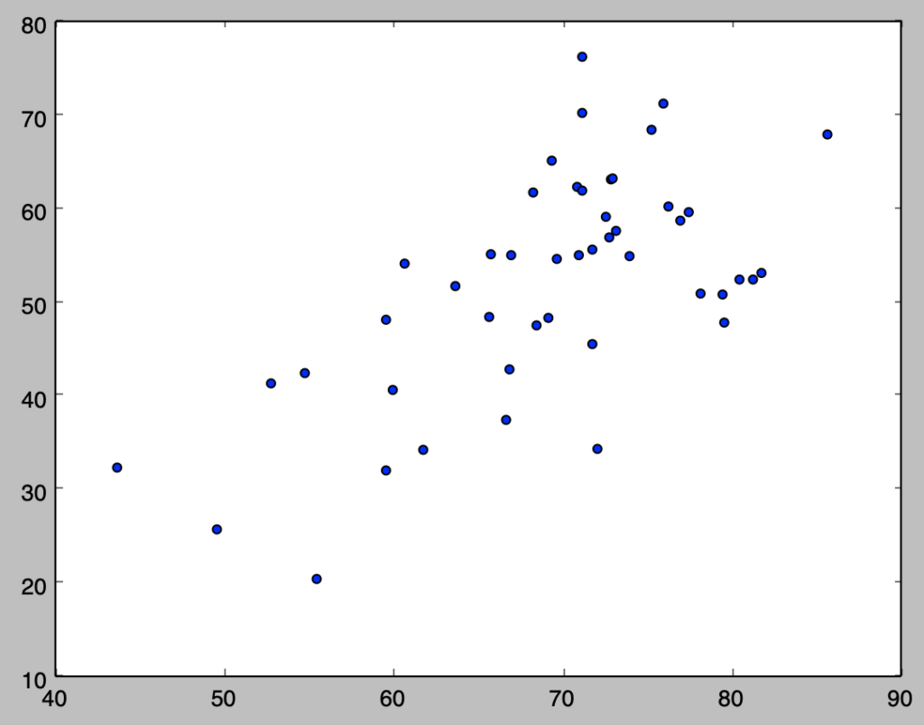
得票率をyとする方が良いと思われたので、逆の順序で作成を行った。
・相関係数の計算
x = np.array([52.8, 71.2, 72.6, 63.7, 81.3, 81.8, 70.9, 74.0, 73.2, 72.9, 66.7, 65.7, 43.7, 55.5, 79.6, 85.7, 75.3, 80.5, 73.0, 77.0, 77.5, 69.2, 60.0, 78.2, 79.5, 61.8, 49.6, 59.6, 72.1, 71.0, 76.3, 72.8, 71.8, 60.7, 67.0, 71.8, 71.2, 68.3, 68.5, 54.8, 76.0, 65.8, 69.4, 66.9, 69.7, 71.2, 59.6])
y = np.array([41.4, 76.3, 59.2, 51.8, 52.5, 53.2, 62.4, 55.0, 57.7, 63.2, 37.5, 48.5, 32.4, 20.5, 47.9, 68.0, 68.5, 52.5, 63.3, 58.8, 59.7, 48.4, 40.7, 51.0, 50.9, 34.3, 25.8, 32.1, 34.4, 55.1, 60.3, 57.0, 45.6, 54.2, 55.1, 55.7, 70.3, 61.8, 47.6, 42.5, 71.3, 55.2, 65.2, 42.9, 54.7, 62.0, 48.2])

r = np.sum((x-np.mean(x))*(y-np.mean(y)))/(np.sqrt(np.sum((x-np.mean(x))**2))*np.sqrt(np.sum((y-np.mean(y))**2)))

print("correlation coef: {:.3f}".format(r))
・実行結果
> print("correlation coef: {:.3f}".format(r))
correlation coef: 0.637
問題3.2の解答例
問題3.3の解答例
下記を実行することで、スピアマンの順位相関係数とケンドールの順位相関係数に基づく相関行列を作成することができる。
import numpy as np

x = np.array([[1., 1., 8., 20.], [2., 5., 3., 1.], [3., 2., 1., 4.], [4., 3., 4., 2.], [5., 6., 2., 6.], [6., 7., 5., 3.], [7., 15., 11., 12.], [8., 8., 7., 17.], [9., 4., 15., 8.], [10., 11., 9., 5.], [11., 10., 6., 18], [12., 14., 13., 13.], [13., 18., 10., 23.], [14., 13., 22., 26.], [15., 22., 12., 29.], [16., 24., 14., 15.], [17., 16., 18., 16.], [18., 19., 19., 9.], [19., 30., 17., 10.], [20., 9., 22., 11.], [21., 25., 16., 30.], [22., 17., 24., 7.], [23., 26., 21., 27.], [24., 23., 20., 19.], [25., 12., 28., 14.], [26., 20., 30., 21.], [27., 28., 25., 28.], [28., 21., 26., 24.], [29., 27., 27., 22.], [30., 29., 29., 25]])

cor_mat_spearman = np.zeros([x.shape[1],x.shape[1]])
cor_mat_kendall = np.zeros([x.shape[1],x.shape[1]])

for i in range(x.shape[1]):
    for j in range(x.shape[1]):
        cor_mat_spearman[i,j] = 1. - 6.*np.sum((x[:,i]-x[:,j])**2)/(x.shape[0]*(x.shape[0]**2-1))
        P, N = 0., 0.
        for k in range(x.shape[0]):
            for l in range(k+1,x.shape[0]):
                if (x[k,i]-x[l,i])*(x[k,j]-x[l,j])>=0:
                    P += 1.
                else:
                    N += 1.
        cor_mat_kendall[i,j] = 2*(P-N)/(x.shape[0]*(x.shape[0]-1.))

print("・Spearman Correlation:")
print(cor_mat_spearman)
print("・Kendall Correlation:")
print(cor_mat_kendall)
・実行結果
・Spearman Correlation:
[[ 1.          0.82157953  0.9272525   0.59332592]
 [ 0.82157953  1.          0.67185762  0.63737486]
 [ 0.9272525   0.67185762  1.          0.53437152]
 [ 0.59332592  0.63737486  0.53437152  1.        ]]
・Kendall Correlation:
[[ 1.          0.66436782  0.77011494  0.43908046]
 [ 0.66436782  1.          0.50344828  0.46206897]
 [ 0.77011494  0.50344828  1.          0.36091954]
 [ 0.43908046  0.46206897  0.36091954  1.        ]]
問題3.4の解答例
i)
巻末の解答では一様乱数が得られる前提なので、以下、numpy.random.randを用いて一様乱数は得られる前提で考える。なお、一様乱数が得られない場合は、乗算合同法などを用いればよい。
下記を実行することで[1, 11]に属する整数の乱数を生成することができる。
import numpy as np

np.random.seed(0)

rand_x = np.random.rand(100)
rand_x_int = np.zeros(100)
for i in range(11):
    rand_x_int[rand_x>i/11.] = i+1

print(rand_x_int)
・実行結果
[  7.   8.   7.   6.   5.   8.   5.  10.  11.   5.   9.   6.   7.  11.   1.
   1.   1.  10.   9.  10.  11.   9.   6.   9.   2.   8.   2.  11.   6.   5.
   3.   9.   6.   7.   1.   7.   7.   7.  11.   8.   4.   5.   8.   1.   8.
   8.   3.   2.   4.   5.   7.   5.  11.   2.   3.   2.   8.   3.   6.   3.
   2.   2.   8.   2.   3.   5.  10.   2.  10.   2.  11.   6.  11.   7.   9.
   1.   4.   2.   4.   2.   4.   5.   1.   8.   7.   3.   6.   2.   7.  11.
   4.   8.   2.   8.   4.   3.   7.   1.  10.   1.]
ⅱ)
下記を実行することで相関係数の計算を行うことができる。
import numpy as np

np.random.seed(0)

x = np.array([71., 68., 66., 67., 70., 71., 70., 73., 72., 65., 66.])
y = np.array([69., 64., 65., 63., 65., 62., 65., 64., 66., 59., 62.])
x_, y_ = np.zeros(11), np.zeros(11)

rand_idx = np.random.rand(11)
rand_idx_int = np.zeros(11)
for i in range(11):
    rand_idx_int[rand_idx>i/11.] = i+1

for i in range(11):
    x_[i] = x[rand_idx_int[i]-1]
    y_[i] = y[rand_idx_int[i]-1]

r = np.sum((x_-np.mean(x_))*(y_-np.mean(y_)))/np.sqrt(np.sum((x_-np.mean(x_))**2) * np.sum((y_-np.mean(y_))**2))

print("Correlation coef: {:.3f}".format(r))
・実行結果
> print("Correlation coef: {:.3f}".format(r))
Correlation coef: 0.678
ⅲ)
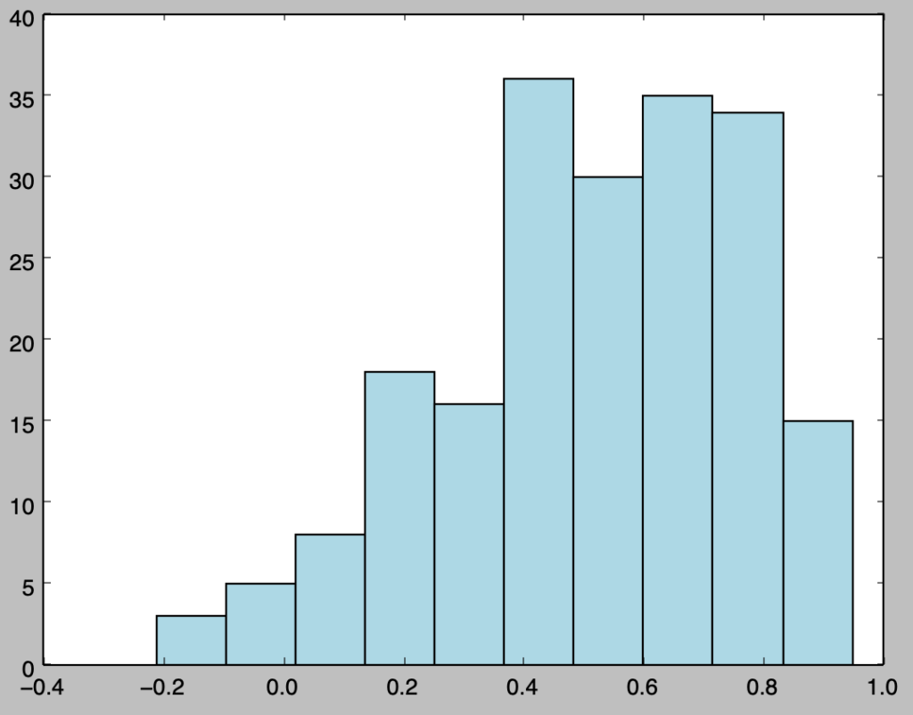
ブートストラップ法に基づくヒストグラムは下記を実行することで作成できる。
import numpy as np
import matplotlib.pyplot as plt

np.random.seed(0)

x = np.array([71., 68., 66., 67., 70., 71., 70., 73., 72., 65., 66.])
y = np.array([69., 64., 65., 63., 65., 62., 65., 64., 66., 59., 62.])
x_, y_ = np.zeros(11), np.zeros(11)

r = np.zeros(200)

for i in range(r.shape[0]):
    rand_idx = np.random.rand(11)
    rand_idx_int = np.zeros(11)

    for j in range(11):
        rand_idx_int[rand_idx>j/11.] = j+1

    for j in range(11):
        x_[j] = x[rand_idx_int[j]-1]
        y_[j] = y[rand_idx_int[j]-1]
    r[i] = np.sum((x_-np.mean(x_))*(y_-np.mean(y_)))/np.sqrt(np.sum((x_-np.mean(x_))**2) * np.sum((y_-np.mean(y_))**2))

plt.hist(r, color="lightblue")
plt.show()
・実行結果
[…] […]