
数式だけの解説ではわかりにくい場合もあると思われるので、統計学の手法や関連する概念をPythonのプログラミングで表現します。当記事では時系列解析(Time-series Analysis)の理解にあたって、AR過程、MA過程、コレログラムなどのPythonでの実装を取り扱いました。
・Pythonを用いた統計学のプログラミングまとめ
https://www.hello-statisticians.com/stat_program
Contents
ARMA過程・共分散定常
AR過程
$$
\large
\begin{align}
y_t = c + \phi_1 y_{t-1} + u_t \quad (1)
\end{align}
$$
系列$\{y_t\}$を上記のような$AR(1)$過程を元に表現することを考える。ここで系列$\{u_t\}$には平均$0$、分散$\sigma^2$のホワイトノイズを考える。以下、ここで定義した式を元に$AR(1)$過程の生成と、期待値・自己共分散の計算に関して取り扱う。
AR過程の生成
式$(1)$に対し、$c=5$、$\phi_1=\{0, 0.5, 0.7\}$、$y_0=2$、ホワイトノイズの分散を$\sigma^2=1$と設定するとき、下記のように$AR(1)$過程の生成を行うことができる。
import numpy as np
from scipy import stats
import matplotlib.pyplot as plt

np.random.seed(0)

c = 5.
phi = np.array([0, 0.5, 0.7])
x = np.arange(0., 100., 1.)
y = np.zeros([100,3])
y[0,:] = 2*np.ones(3)

for i in range(1, y.shape[0]):
     y[i, :] = c + phi*y[i-1, :] + stats.norm.rvs(0,size=3)

for i in range(3):
    plt.plot(x, y[:,i])

plt.show()
・実行結果
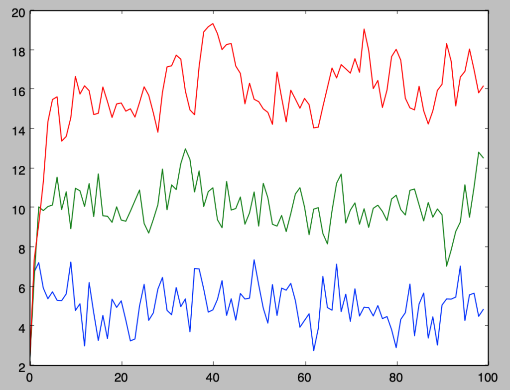
上記はどれも$\phi_1$に関して生成を行ったので、$\phi_1=-0.7$に関しても確認を行う。
import numpy as np
from scipy import stats
import matplotlib.pyplot as plt

np.random.seed(0)

c = 5.
phi = np.array([-0.7])
x = np.arange(0., 100., 1.)
y = np.zeros([100,1])
y[0,:] = 2*np.ones(1)

for i in range(1, y.shape[0]):
     y[i, :] = c + phi*y[i-1, :] + stats.norm.rvs(0,size=1)

for i in range(1):
    plt.plot(x, y[:,i])

plt.show()
・実行結果
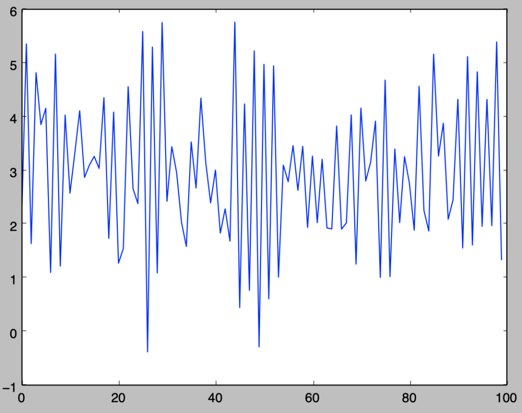
$\phi_1$の値が負の場合、$y_t-\bar{y}$と$y_{t-1}-\bar{y}$が異符号になりやすいことを意味するので、$\phi_1 \geq 0$のときに比べて値の上下がしやすくなることに注意しておくと良い。
AR過程の期待値、自己共分散
・期待値の計算
$$
\large
\begin{align}
E[Y_t] = \frac{c}{1-\phi_1} \quad (2)
\end{align}
$$
$(1)$式で定義を行った$AR(1)$過程は、$|\phi_1|<1$のとき、上記のような期待値を考えることができる。ここでは$Y_t$と$y_t$は確率変数とその実現値のように表記を使い分けた。
以下、前項で生成した系列の平均が$(2)$式に一致するかの確認を行う。
import numpy as np
from scipy import stats
import matplotlib.pyplot as plt

np.random.seed(0)

c = 5.
phi = np.array([-0.7, 0, 0.3, 0.5, 0.7])
y = np.zeros([110,5])
y[0,:] = 2*np.ones(5)

for i in range(1, y.shape[0]):
     y[i, :] = c + phi*y[i-1, :] + stats.norm.rvs(0,size=5)

print(np.mean(y[:10,:],axis=0))
print(np.mean(y[10:,:],axis=0))
print(c/(1.-phi))
・実行結果
> print(np.mean(y[:10,:],axis=0))
[  2.63929888   5.21864106   6.56471946   8.84802352  13.34988176]
> print(np.mean(y[10:,:],axis=0))
[  2.88815475   4.9228795    7.04124409   9.65664408  17.04847973]
> print(c/(1.-phi))
[  2.94117647   5.           7.14285714  10.          16.66666667]
実行結果を確認すると、$(2)$式が概ね正しいことが確認できる。また、$110$個の値を生成し、$1$つ目から$100$個と、$11$個目の$100$個を元に平均の比較を行った。これにより初期値により依存しない定常状態での計算が行うことができ、実行結果からもそのことを反映していることが確認できる。
・分散、1次の自己共分散の計算
$$
\large
\begin{align}
\gamma_{0} &= \frac{\sigma^2}{1-\phi_{1}^{2}} \quad (3) \\
\gamma_{1} &= \phi_{1} \frac{\sigma^2}{1-\phi_{1}^{2}} \quad (4)
\end{align}
$$
$(1)$式で定義を行った$AR(1)$過程は、$|\phi_1|<1$のとき、上記のような分散$\gamma_{0}$と1次の自己共分散$\gamma_{1}$を考えることができる。ここでは$Y_t$と$y_t$は確率変数とその実現値のように表記を使い分けた。
以下、前項で生成した系列の分散と1次の自己共分散が$(3), (4)$式に一致するかの確認を行う。
np.random.seed(0)

c = 5.
phi = np.array([-0.7, 0, 0.3, 0.5, 0.7])
y = np.zeros([110,5])
y[0,:] = 2*np.ones(5)

for i in range(1, y.shape[0]):
     y[i, :] = c + phi*y[i-1, :] + stats.norm.rvs(0,size=5)

y_t = y[10:,:]
y_t_1 = y[9:109,:]
est_gamma_0 = np.sum((y_t-np.mean(y_t,axis=0))**2, axis=0)/y_t.shape[0]
est_gamma_1 = np.sum((y_t-np.mean(y_t,axis=0))*(y_t_1-np.mean(y_t_1,axis=0)), axis=0)/y_t.shape[0]
pop_gamma_0 = 1./(1.-phi**2)
pop_gamma_1 = phi*1./(1.-phi**2)

print("population gamma_0: {}".format(pop_gamma_0))
print("estimated gamma_0: {}".format(est_gamma_0))
print("===")
print("population gamma_1: {}".format(pop_gamma_1))
print("estimated gamma_1: {}".format(est_gamma_1))
・実行結果
population gamma_0: [ 1.96078431  1.          1.0989011   1.33333333  1.96078431]
estimated gamma_0: [ 1.96412646  0.89642751  1.17330429  1.63729046  1.53448253]
===
population gamma_1: [-1.37254902  0.          0.32967033  0.66666667  1.37254902]
estimated gamma_1: [-1.41202877 0.00415049 0.37561853 1.01843126 0.9910005 ]以下生成するyの要素の数を増やして同様の確認を行う。
np.random.seed(0)

c = 5.
phi = np.array([-0.7, 0, 0.3, 0.5, 0.7])
y = np.zeros([10100,5])
y[0,:] = 2*np.ones(5)

for i in range(1, y.shape[0]):
     y[i, :] = c + phi*y[i-1, :] + stats.norm.rvs(0,size=5)

y_t = y[100:,:]
y_t_1 = y[99:10099,:]
est_gamma_0 = np.sum((y_t-np.mean(y_t,axis=0))**2, axis=0)/y_t.shape[0]
est_gamma_1 = np.sum((y_t-np.mean(y_t,axis=0))*(y_t_1-np.mean(y_t_1,axis=0)), axis=0)/y_t.shape[0]
pop_gamma_0 = 1./(1.-phi**2)
pop_gamma_1 = phi*1./(1.-phi**2)

print("population gamma_0: {}".format(pop_gamma_0))
print("estimated gamma_0: {}".format(est_gamma_0))
print("===")
print("population gamma_1: {}".format(pop_gamma_1))
print("estimated gamma_1: {}".format(est_gamma_1))
・実行結果
population gamma_0: [ 1.96078431  1.          1.0989011   1.33333333  1.96078431]
estimated gamma_0: [ 1.97233741  1.0029984   1.0905944   1.32661458  1.97339705]
===
population gamma_1: [-1.37254902  0.          0.32967033  0.66666667  1.37254902]
estimated gamma_1: [-1.38088791  0.01162902  0.32819272  0.66243822  1.40465808]
MA過程
$$
\large
\begin{align}
y_t = \mu + u_t + \theta_{1} u_{t-1} \quad (5)
\end{align}
$$
系列${y_t}$を上記のような$MA(1)$過程を元に表現することを考える。ここで系列${u_t}$には平均$0$、分散$\sigma^2$のホワイトノイズを考える。以下、ここで定義した式を元に$MA(1)$過程の生成と、期待値・自己共分散の計算に関して取り扱う。
MA過程の生成
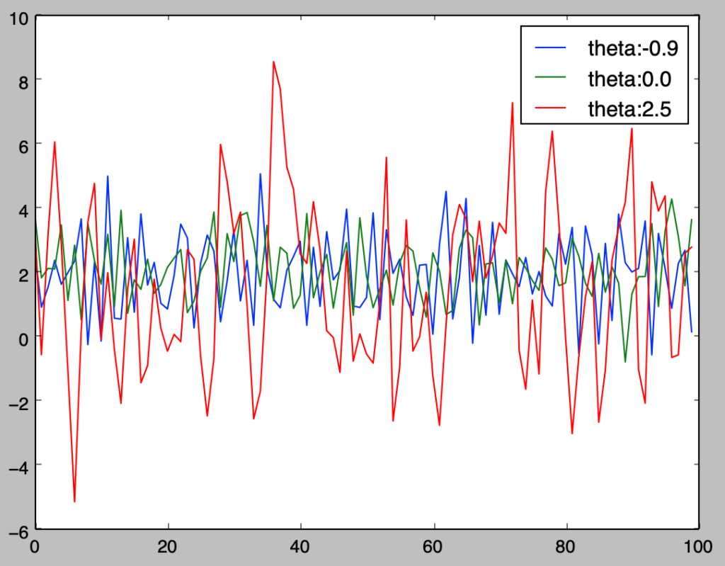
式$(5)$に対し、$\mu=2$、$\phi_1=\{-0.9, 0, 2.5\}$、ホワイトノイズの分散を$\sigma^2=1$と設定するとき、下記のように$MA(1)$過程の生成を行うことができる。
import numpy as np
from scipy import stats
import matplotlib.pyplot as plt

np.random.seed(0)

mu = 2
theta = np.array([-0.9, 0., 2.5])
x = np.arange(0., 100., 1.)
y = np.zeros([100,3])

u_t_1 = stats.norm.rvs(0,size=3)
for i in range(y.shape[0]):
    u_t = stats.norm.rvs(0,size=3)
    y[i, :] = mu + u_t + theta*u_t_1
    u_t_1 = u_t

for i in range(3):
    plt.plot(x, y[:,i],label="theta:{}".format(theta[i]))

plt.legend()
plt.show()
・実行結果
MA過程の期待値、自己共分散
・期待値の計算
$$
\large
\begin{align}
E[Y_t] = \mu \quad (6)
\end{align}
$$
$(5)$式で定義を行った$MA(1)$過程は、上記のような期待値を考えることができる。ここでは$Y_t$と$y_t$は確率変数とその実現値のように表記を使い分けた。
以下、前項で生成した系列の平均が$(6)$式に一致するかの確認を行う。
import numpy as np
from scipy import stats
import matplotlib.pyplot as plt

np.random.seed(0)

mu = 2
theta = np.array([-0.9, 0., 2.5])
y = np.zeros([100,3])

u_t_1 = stats.norm.rvs(0,size=3)
for i in range(y.shape[0]):
    u_t = stats.norm.rvs(0,size=3)
    y[i, :] = mu + u_t + theta*u_t_1
    u_t_1 = u_t

print(np.mean(y,axis=0))
print(mu)
・実行結果
> print(np.mean(y,axis=0))
[ 1.97934626  2.11883204  1.55438665]
> print(mu)
2
・分散、1次の自己共分散の計算
$$
\large
\begin{align}
\gamma_{0} &= (1+\theta_{1}^{2}) \sigma^2 \quad (7) \\
\gamma_{1} &= \theta_1 \sigma^2 \quad (8)
\end{align}
$$
$(5)$式で定義を行った$AR(1)$過程は、上記のような分散$\gamma_{0}$と1次の自己共分散$\gamma_{1}$を考えることができる。ここでは$Y_t$と$y_t$は確率変数とその実現値のように表記を使い分けた。
以下、前項で生成した系列の分散と1次の自己共分散が$(7), (8)$式に一致するかの確認を行う。
np.random.seed(0)

mu = 2
theta = np.array([-0.9, 0., 2.5])
y = np.zeros([101,3])

u_t_1 = stats.norm.rvs(0,size=3)
for i in range(y.shape[0]):
    u_t = stats.norm.rvs(0,size=3)
    y[i, :] = mu + u_t + theta*u_t_1
    u_t_1 = u_t

y_t = y[1:,:]
y_t_1 = y[:-1,:]
est_gamma_0 = np.sum((y_t-np.mean(y_t,axis=0))**2, axis=0)/y_t.shape[0]
est_gamma_1 = np.sum((y_t-np.mean(y_t,axis=0))*(y_t_1-np.mean(y_t_1,axis=0)), axis=0)/y_t.shape[0]
pop_gamma_0 = 1.+theta**2
pop_gamma_1 = theta

print("population gamma_0: {}".format(pop_gamma_0))
print("estimated gamma_0: {}".format(est_gamma_0))
print("===")
print("population gamma_1: {}".format(pop_gamma_1))
print("estimated gamma_1: {}".format(est_gamma_1))
・実行結果
population gamma_0: [ 1.81  1.    7.25]
estimated gamma_0: [ 1.5933599   0.95971088  7.29452229]
===
population gamma_1: [-0.9  0.   2.5]
estimated gamma_1: [-0.75201479 -0.13068008 2.62407484]以下生成するyの要素の数を増やして同様の確認を行う。
np.random.seed(0)

mu = 2
theta = np.array([-0.9, 0., 2.5])
y = np.zeros([10100,3])

u_t_1 = stats.norm.rvs(0,size=3)
for i in range(y.shape[0]):
    u_t = stats.norm.rvs(0,size=3)
    y[i, :] = mu + u_t + theta*u_t_1
    u_t_1 = u_t

y_t = y[100:,:]
y_t_1 = y[99:10099,:]
est_gamma_0 = np.sum((y_t-np.mean(y_t,axis=0))**2, axis=0)/y_t.shape[0]
est_gamma_1 = np.sum((y_t-np.mean(y_t,axis=0))*(y_t_1-np.mean(y_t_1,axis=0)), axis=0)/y_t.shape[0]
pop_gamma_0 = 1.+theta**2
pop_gamma_1 = theta

print("population gamma_0: {}".format(pop_gamma_0))
print("estimated gamma_0: {}".format(est_gamma_0))
print("===")
print("population gamma_1: {}".format(pop_gamma_1))
print("estimated gamma_1: {}".format(est_gamma_1))
・実行結果
population gamma_0: [ 1.81  1.    7.25]
estimated gamma_0: [ 1.82644804  0.9895947   7.04606486]
===
population gamma_1: [-0.9  0.   2.5]
estimated gamma_1: [ -9.48202031e-01   2.08049843e-03   2.39463923e+00]
共分散定常
コレログラム
AR過程のコレログラム
$$
\large
\begin{align}
y_t = c + \phi_1 y_{t-1} + u_t \quad (1)
\end{align}
$$
前節で取り扱った上記のように表される$AR$過程の$h$次の自己共分散は下記のように表される。
$$
\large
\begin{align}
\gamma_{h} &= \phi_{1}^{h} \frac{\sigma^2}{1-\phi_{1}^{2}} \quad (9)
\end{align}
$$
上記の式に対して、$h$はラグであり、$h=0$の$0$次の自己共分散は分散を表すと考える。
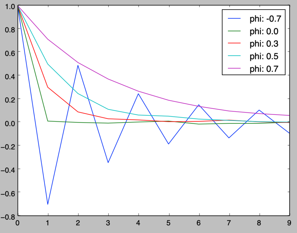
以下、前節で取り扱った$AR$過程と同様の例を用いて、標本自己相関係数を元にコレログラムの作成を行い、$(9)$式との比較を行う。
import numpy as np
from scipy import stats
import matplotlib.pyplot as plt

np.random.seed(0)

c = 5.
h = np.arange(0,10,1)
phi = np.array([-0.7, 0, 0.3, 0.5, 0.7])
y = np.zeros([10100,5])
y[0,:] = 2*np.ones(5)

for i in range(1, y.shape[0]):
     y[i, :] = c + phi*y[i-1, :] + stats.norm.rvs(0,size=5)

y_t_h = list()
est_gamma, pop_gamma = np.zeros([10,5]), np.zeros([10,5])

for i in range(h.shape[0]):
    y_t_h.append(y[(100-i):(10100-i),:])
    est_gamma[i,:] = np.sum((y_t_h[0]-np.mean(y_t_h[0],axis=0))*(y_t_h[i]-np.mean(y_t_h[i],axis=0)), axis=0)/y_t_h[0].shape[0]
    pop_gamma[i,:] = (phi**i)/(1.-phi**2)

print("population gamma_h: {}".format(pop_gamma))
print("estimated gamma_h: {}".format(est_gamma))

for i in range(phi.shape[0]):
    plt.plot(h,est_gamma[:,i]/est_gamma[0,i], label="phi: {}".format(phi[i]))

plt.legend()
plt.show()
・実行結果
MA過程のコレログラム
$$
\large
\begin{align}
y_t = \mu + u_t + \theta_{1} u_{t-1} \quad (5)
\end{align}
$$
前節で取り扱った上記のように表される$MA$過程の$h$次の自己共分散は下記のように表される。
$$
\large
\begin{align}
\gamma_{h} &= (1+\theta_{1}^{2}) \sigma^2, \quad h=0 \\
&= \theta_{1} \sigma^2, \quad h=1 \\
&= 0, \quad h>1 \quad (10)
\end{align}
$$
上記の式に対して、$h$はラグであり、$h=0$の$0$次の自己共分散は分散を表すと考える。
以下、前節で取り扱った$MA$過程と同様の例を用いて、標本自己相関係数を元にコレログラムの作成を行い、$(10)$式との比較を行う。
np.random.seed(0)

mu = 2
h = np.arange(0,10,1)
theta = np.array([-0.9, 0., 2.5])
y = np.zeros([10100,3])

u_t_1 = stats.norm.rvs(0,size=3)
for i in range(y.shape[0]):
    u_t = stats.norm.rvs(0,size=3)
    y[i, :] = mu + u_t + theta*u_t_1
    u_t_1 = u_t

y_t_h = list()
est_gamma, pop_gamma = np.zeros([10,3]), np.zeros([10,3])
pop_gamma[0,:], pop_gamma[1,:] = 1+theta**2, theta

for i in range(h.shape[0]):
    y_t_h.append(y[(100-i):(10100-i),:])
    est_gamma[i,:] = np.sum((y_t_h[0]-np.mean(y_t_h[0],axis=0))*(y_t_h[i]-np.mean(y_t_h[i],axis=0)), axis=0)/y_t_h[0].shape[0]

print("population gamma_h: {}".format(pop_gamma))
print("estimated gamma_h: {}".format(est_gamma))

for i in range(theta.shape[0]):
    plt.plot(h,est_gamma[:,i]/est_gamma[0,i], label="phi: {}".format(theta[i]))

plt.legend()
plt.show()
・実行結果
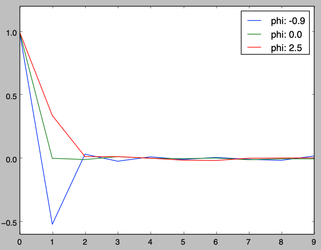
上記の結果は、$MA(1)$過程の$h>1$での自己共分散$\gamma_{h}$が$0$であることに基づくと考えることができる。
ホワイトノイズ
独立と無相関
独立と無相関に関しては混同しがちだが、独立は確率分布に関する前提である一方で無相関は期待値に関する前提であり、それぞれは異なることを把握しておく必要がある。
・独立
$$
\large
\begin{align}
p(x,y) = p(x)p(y)
\end{align}
$$
・無相関
$$
\large
\begin{align}
E[XY] = E[X]E[Y]
\end{align}
$$
上記で表したように、独立は確率分布に関する仮定、無相関は期待値に関する仮定である。$p(x,y)=p(x)p(y) \implies E[XY]=E[X]E[Y]$であるが逆は成立しないことを抑えておく必要がある。独立ならば必ず無相関であるが、無相関でも独立であるとは限らないと考えておくと良い。
以下、「独立かつ無相関」と「無相関であるが独立ではない」事例に関して確認を行う。
import numpy as np
import matplotlib.pyplot as plt

x = np.repeat(np.arange(1.,7.,1.),6)
y = x.reshape([6,6]).T.reshape(36)

x_, y_ = np.repeat(np.arange(1.,7.,1.),6), x.reshape([6,6]).T.reshape(36)
for i in range(6):
    x_[6*i] = 2*(x_[6*i]-3.5)+3.5
    x_[6*i+2] = 0.5*(x_[6*i+2]-3.5)+3.5
    x_[6*i+5] = 2.5*(x_[6*i+5]-3.5)+3.5

cov_xy = np.sum((x-np.mean(x))*(y-np.mean(y)))
cov_xy_ = np.sum((x_-np.mean(x_))*(y_-np.mean(y_)))

print(cov_xy)
print(cov_xy_)

plt.scatter(x_,y_)
plt.show()
・実行結果
> print(cov_xy)
0.0
> print(cov_xy_)
0.0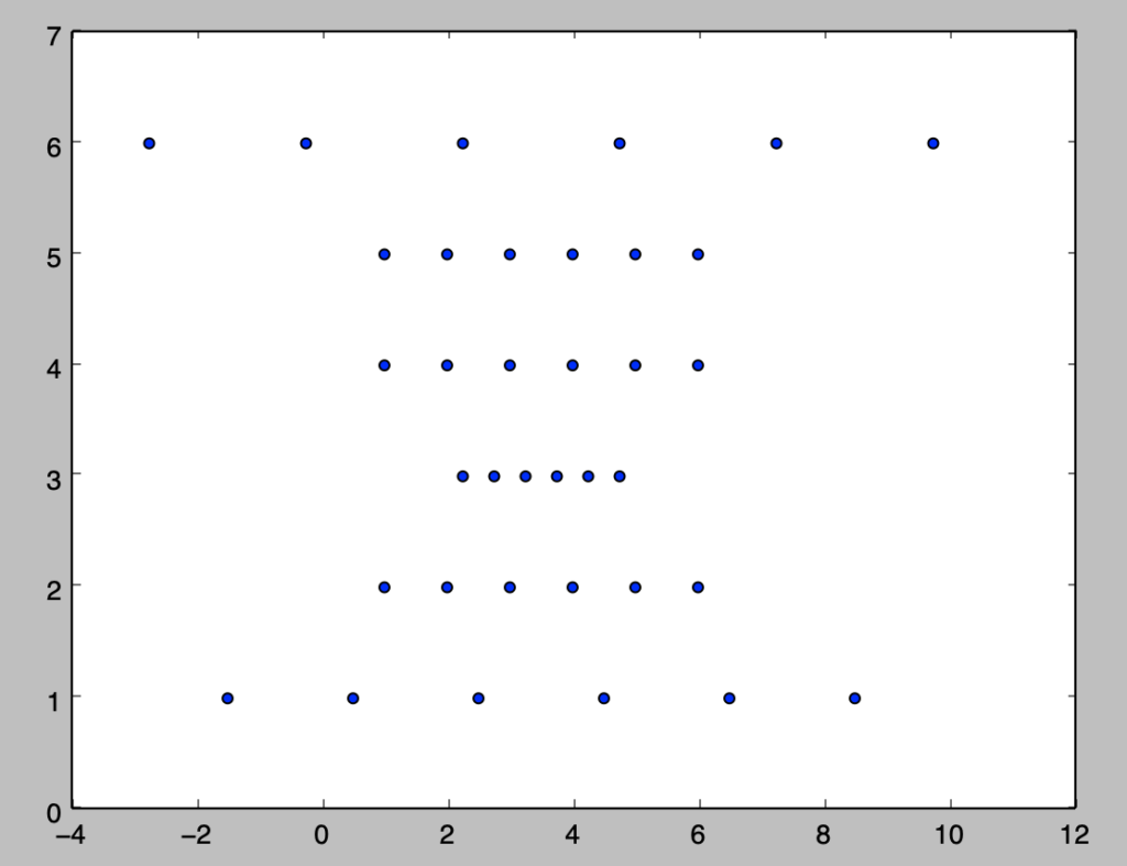
x_とy_は無相関である一方で、x_の値がy_の値によって変化するので独立ではない。このように無相関だが独立ではない場合もあることに注意が必要である。
独立と無相関に関しては下記でも取り扱いを行った。
https://www.hello-statisticians.com/explain-books-cat/toukeigakunyuumon-akahon/ch7_practice.html#73
$i.i.d.$以外のホワイトノイズの例
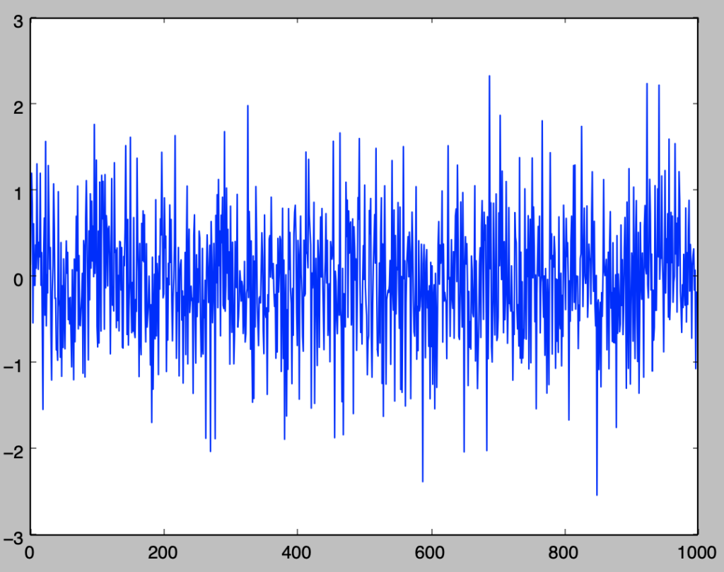
ホワイトノイズの簡単な例には$u_t \sim N(0,1), \quad i.i.d.,$が考えられるが、ここでは$i.i.d.$以外のホワイトノイズの例に関して確認を行う。
import numpy as np
import matplotlib.pyplot as plt
from scipy import stats

np.random.seed(0)

t = np.arange(0,1000,1)
u = np.zeros(1000)
sigma = 1
for i in range(u.shape[0]):
    u[i] = stats.norm.rvs(loc=0,scale=sigma)
    sigma = 1./(np.abs(u[i])+1.)

plt.plot(t,u)
plt.show()
・実行結果
ここで、上記のようにuを生成する場合のコレログラムを作成し、ホワイトノイズであることの確認を行う。
np.random.seed(0)

t = np.arange(0,10100,1)
u = np.zeros(10100)
sigma = 1
for i in range(u.shape[0]):
    u[i] = stats.norm.rvs(loc=0,scale=sigma)
    sigma = 1./(np.abs(u[i])+1.)

h = np.arange(0,10,1)
u_t_h = list()
est_gamma = np.zeros(10)

for i in range(h.shape[0]):
    u_t_h.append(u[(100-i):(10100-i)])
    est_gamma[i] = np.sum((u_t_h[0]-np.mean(u_t_h[0]))*(u_t_h[i]-np.mean(u_t_h[i])))/u_t_h[0].shape[0]

print(np.mean(u))

plt.bar(h,est_gamma)
plt.show()
・実行結果
> print(np.mean(u))
-0.0106528437504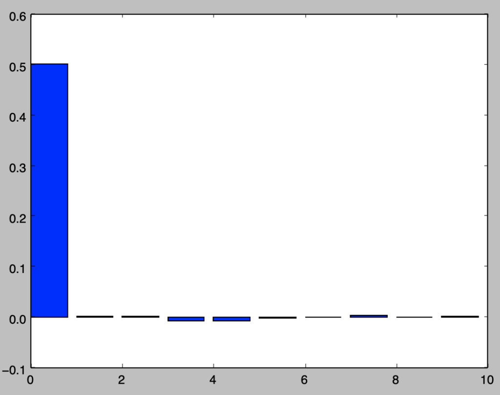
上記より平均と$h>0$での自己共分散が$0$であることが確認できるので、ここで生成されたuがホワイトノイズであると考えることができる。
スペクトラム
検定
単位根検定・ディッキーフラー検定
ダービン・ワトソン検定
ダービン・ワトソン検定(Durbin Watson test)は$u_t$などで表される誤差項に自己相関が存在するかどうかの確認を行う検定である。
$$
\large
\begin{align}
u_{t} = \rho u_{t-1} + \epsilon_{t}
\end{align}
$$
ダービン・ワトソン検定では上記のように誤差項$u_t$が$AR(1)$過程に従うことを仮定する。ここで下記のような帰無仮説$H_0$と対立仮説$H_1$を考える。
$$
\large
\begin{align}
H_0: \quad \rho = 0 \\
H_1: \quad \rho > 0
\end{align}
$$
上記の仮説の検定にあたって、得られた残差$\hat{u}_t$を用いて下記のようにダービン・ワトソン比$DW$を検定統計量に考える。
$$
\large
\begin{align}
DW &= \frac{\sum_{t=2}^{T} (\hat{u}_{t}-\hat{u}_{t-1})^2}{\sum_{t=1}^{T} \hat{u}_{t}^2} = \frac{\sum_{t=2}^{T} \hat{u}_{t}^{2}+\sum_{t=2}^{T} \hat{u}_{t-1}^{2}-2\sum_{t=2}^{T} \hat{u}_{t}\hat{u}_{t-1}}{\sum_{t=1}^{T} \hat{u}_{t}^2} \\
& \simeq 2 \left( 1 – \frac{\sum_{t=2}^{T} \hat{u}_{t}\hat{u}_{t-1}}{\sum_{t=1}^{T} \hat{u}_{t}^2} \right) = 2(1-\hat{\gamma}_1)
\end{align}
$$
上記で定義を行ったダービン・ワトソン比が$2$に近いとき、帰無仮説を受容し、$2$より十分小さな場合に帰無仮説の棄却を行う。
[…] 下記などで取り扱いを行った。https://www.hello-statisticians.com/python/stat_program3.html […]