曲線を媒介変数表示する場合、微小区間に三平方の定理を適用し積分を行うことで、曲線の長さを計算することができます。当記事では基本的な公式を確認したのちに、計算の具体例を考えるにあたって、アステロイド、カージオイド、アルキメデスの螺旋などの曲線の長さに関して取り扱います。
作成にあたっては「チャート式シリーズ 大学教養 微分積分」の第$4$章「積分」を主に参考にしました。
・数学まとめ
https://www.hello-statisticians.com/math_basic
曲線の長さの公式
曲線の媒介変数表示
$2$変数$x(t),y(t)$を$t$の式で表すことを考える。たとえば半径$a>0$の円の第$1$象限での軌跡は下記のように表すことができる。
$$
\large
\begin{align}
x(t) &= a \cos{t} \\
y(t) &= a \sin{t} \\
0 \leq & t \leq \frac{\pi}{2}
\end{align}
$$
上記が半径$a$の円を表すことは下記のように$x(t)^2+y(t)^2$を計算することで確認することができる。
$$
\large
\begin{align}
x(t)^2 + y(t)^2 &= a^2 \cos^{2}{t} + a^2 \sin^{2}{t} \\
&= a^2 ( \cos^{2}{t} + \sin^{2}{t} ) \\
&= a^2
\end{align}
$$
半径$r$の円の方程式が$x^2+y^2=r^2$であることから、$x(t) = a \cos{t}, y(t) = a \sin{t}$が円を描くということが確認できる。
積分を用いた曲線の長さの公式
$\alpha \leq t \leq \beta$の範囲で$t$が動くとき、$x(t),y(t)$が描く曲線の長さを$L$とおくと、$L$は下記のように計算できる。
$$
\large
\begin{align}
L = \int_{\alpha}^{\beta} \sqrt{\left( \frac{dx(t)}{dt} \right)^2 + \left( \frac{dy(t)}{dt} \right)^2} dt \quad (1)
\end{align}
$$
上記の公式は「微小区間に関して三平方の定理を適用し、積分を行なうことで長さが計算できる」と解釈すると良い。
使用例
以下、「チャート式シリーズ 大学教養 微分積分」の例題の確認を行う。
基本例題$088$
$$
\large
\begin{align}
x(t) &= a \cos^{3}{t} \\
y(t) &= a \sin^{3}{t} \\
0 \leq & t \leq \frac{\pi}{2}
\end{align}
$$
以下、上記で表される曲線の長さ$L$の計算を行う。
$$
\large
\begin{align}
\frac{dx(t)}{dt} &= -3a \cos^{2}{t} \sin{t} \\
\frac{dy(t)}{dt} &= 3a \sin^{2}{t} \cos{t}
\end{align}
$$
上記に基づいて$L$は下記のように計算できる。
$$
\large
\begin{align}
L &= \int_{0}^{\frac{\pi}{2}} \sqrt{\left( \frac{dx(t)}{dt} \right)^2 + \left( \frac{dy(t)}{dt} \right)^2} dt \\
&= \int_{0}^{\frac{\pi}{2}} \sqrt{9a^2 \cos^{4}{t} \sin^{2}{t} + 9a^2 \sin^{4}{t} \cos^{2}{t}} dt \\
&= \int_{0}^{\frac{\pi}{2}} \sqrt{9a^2 \cos^{2}{t} \sin^{2}{t}(\cos^{2}{t} + \sin^{2}{t})} dt \\
&= \int_{0}^{\frac{\pi}{2}} \sqrt{9a^2 \cos^{2}{t} \sin^{2}{t}} dt \\
&= \int_{0}^{\frac{\pi}{2}} 3a \cos{t} \sin{t} dt \\
&= \frac{3}{2}a \int_{0}^{\frac{\pi}{2}} \sin{2t} dt \\
&= \frac{3}{2}a \left[ – \frac{1}{2} \cos{2t} \right]_{0}^{\frac{\pi}{2}} \\
&= \frac{3}{2}a
\end{align}
$$
途中計算では$\displaystyle 0 \leq t \leq \frac{\pi}{2}$より、$\cos{t} \geq 0, \sin{t} \geq 0$であることを用いた。
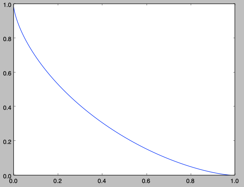
・考察
この問題で取り扱った曲線はアステロイド${}^{3}\sqrt{x^2}+{}^{3}\sqrt{y^2}=a^{2/3}$の第$1$象限に対応する。曲線の直感的な理解ができるように、以下ではPythonを用いて描画を行う。
import numpy as np
import matplotlib.pyplot as plt

a = 1.

t = np.linspace(0,np.pi/2,100)
x = a*np.cos(t)**3
y = a*np.sin(t)**3

plt.plot(x,y)
plt.show()
・実行結果
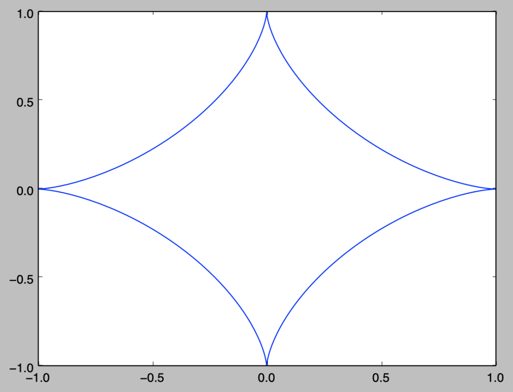
上記は$\displaystyle 0 \leq t \leq \frac{\pi}{2}$で描画を行なったが、$0 \leq t \leq 2 \pi$では下記のように描画できる。
import numpy as np
import matplotlib.pyplot as plt

a = 1.

t = np.linspace(0,2.*np.pi,300)
x = a*np.cos(t)**3
y = a*np.sin(t)**3

plt.plot(x,y)
plt.show()
・実行結果
重要例題$047$
$(x,y) = (r \cos{\theta}, r \sin{\theta})$が成立する際に、極方程式$r=f(\theta), \: \alpha \leq \theta \leq \beta$で表される曲線$C$の長さ$l(C)$は下記のように計算できる。
$$
\large
\begin{align}
l(C) = \int_{\alpha}^{\beta} \sqrt{[f(\theta)]^2+[f'(\theta)]^2} d \theta \quad (2)
\end{align}
$$
以下、前述の$(1)$式を用いて$(2)$式が成立することを示す。$x(\theta) = f(\theta) \cos{\theta}, y(\theta) = f(\theta) \sin{\theta}$であるので、下記のように微分を考えることができる。
$$
\large
\begin{align}
\frac{d x(\theta)}{d \theta} &= f'(\theta) \cos{\theta} – f(\theta) \sin{\theta} \\
\frac{d y(\theta)}{d \theta} &= f'(\theta) \sin{\theta} + f(\theta) \cos{\theta}
\end{align}
$$
よって、$l(C)$は$(1)$式から下記のように計算できる。
$$
\large
\begin{align}
l(C) &= \int_{\alpha}^{\beta} \sqrt{\left( \frac{dx(\theta)}{d \theta} \right)^2 + \left( \frac{dy(\theta)}{d \theta} \right)^2} d \theta \quad (1)’ \\
&= \int_{\alpha}^{\beta} \sqrt{(f'(\theta) \cos{\theta} – f(\theta) \sin{\theta})^2+(f'(\theta) \sin{\theta} + f(\theta) \cos{\theta})^2} d \theta \\
&= \int_{\alpha}^{\beta} \sqrt{f'(\theta)^2(\cos^2{\theta}+\sin^2{\theta}) + f(\theta)^2(\cos^2{\theta}+\sin^2{\theta}) + 2f'(\theta)f(\theta)\cos{\theta}\sin{\theta}(1-1)} d \theta \\
&= \int_{\alpha}^{\beta} \sqrt{f(\theta)^2(\cos^2{\theta}+\sin^2{\theta}) + f'(\theta)^2(\cos^2{\theta}+\sin^2{\theta})} d \theta \\
&= \int_{\alpha}^{\beta} \sqrt{f(\theta)^2 + f'(\theta)^2} d \theta \quad (2)
\end{align}
$$
重要例題$048$
$(1)$ カージオイドの長さ
$$
\large
\begin{align}
r(\theta) &= a(1+\cos{\theta}), \quad 0 \leq \theta \leq 2 \pi, \: a>0 \\
x(\theta) &= r(\theta)\cos{\theta}, \: y(\theta) = r(\theta)\sin{\theta}
\end{align}
$$
カージオイドは上記のように定義される$x(\theta),y(\theta)$の軌跡で表される。この長さを$l(C)$とおく。重要例題$047$で導出した式を用いるにあたって、$r(\theta)$の$\theta$での微分を計算する。
$$
\large
\begin{align}
\frac{dr(\theta)}{d \theta} &= \frac{d}{d \theta} (a(1+\cos{\theta})) \\
&= -a \sin{\theta}
\end{align}
$$
曲線が$y=0$で対称であることから、$l(C)$は下記のように計算できる。
$$
\large
\begin{align}
l(C) &= \int_{0}^{2 \pi} \sqrt{r(\theta)^2 + \left( \frac{dr(\theta)}{d \theta} \right)^2} d \theta \\
&= 2 \int_{0}^{\pi} \sqrt{r(\theta)^2 + \left( \frac{dr(\theta)}{d \theta} \right)^2} d \theta \\
&= 2 \int_{0}^{\pi} \sqrt{a^2(1+\cos{\theta})^2 + a^2 \sin{\theta}^2} d \theta \\
&= 2a \int_{0}^{\pi} \sqrt{(1+\cos^2{\theta}+2\cos{\theta}) + \sin{\theta}^2} d \theta \\
&= 2a \int_{0}^{\pi} \sqrt{2(1+\cos{\theta})} d \theta \\
&= 2a \int_{0}^{\pi} \sqrt{4 \cos^2{\frac{\theta}{2}}} d \theta \\
&= 2a \int_{0}^{\pi} 2 \cos{\frac{\theta}{2}} d \theta \\
&= 2a \left[ 4 \sin{\frac{\theta}{2}} \right]_{0}^{\pi} \\
&= 8a
\end{align}
$$
・考察
カージオイドの直感的な理解ができるように、以下ではPythonを用いて描画を行う。
import numpy as np
import matplotlib.pyplot as plt

a = 1.

theta = np.linspace(0,2*np.pi,300)
r = a*(1+np.cos(theta))

x = r*np.cos(theta)
y = r*np.sin(theta)

plt.ficure(7,7)
plt.plot(x,y)
plt.xlim([-0.7,2.3])
plt.ylim([-1.5,1.5])
plt.show()
・実行結果
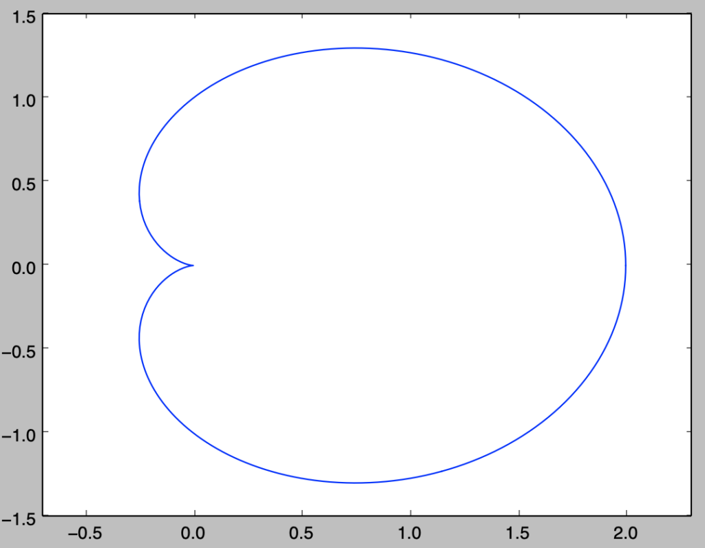
上図は$a=1$で計算したので、図の曲線の長さは$l(C)=8$に対応する。半径$1$の円周の長さは$2 \pi = 6.28…$より、ここで取り扱ったカージオイドは半径$1$の円の円周より長いことが確認できる。このことは図からも大まかに読み取れる。
$(2)$ アルキメデスの螺旋の長さ
$$
\large
\begin{align}
r(\theta) &= a \theta, \quad 0 \leq \theta \leq 2 \pi, \: a>0 \\
x(\theta) &= r(\theta)\cos{\theta}, \: y(\theta) = r(\theta)\sin{\theta}
\end{align}
$$
アルキメデスの螺旋は上記のように定義される$x(\theta),y(\theta)$の軌跡で表される。この長さを$l(C)$とおく。重要例題$047$で導出した式を用いるにあたって、$r(\theta)$の$\theta$での微分を計算する。
$$
\large
\begin{align}
\frac{dr(\theta)}{d \theta} = a
\end{align}
$$
曲線が$y=0$で対称であることから、$l(C)$は下記のように表せる。
$$
\large
\begin{align}
l(C) &= \int_{0}^{2 \pi} \sqrt{r(\theta)^2 + \left( \frac{dr(\theta)}{d \theta} \right)^2} d \theta \\
&= \int_{0}^{2 \pi} \sqrt{a^2 \theta^2 + a^2} d \theta \\
&= a \int_{0}^{2 \pi} \sqrt{1 + \theta^2} d \theta
\end{align}
$$
$l(C)$は下記のように計算できる。
$$
\large
\begin{align}
l(C) &= a \int_{0}^{2 \pi} \sqrt{1 + \theta^2} d \theta \\
&= a \left[ \frac{1}{2} (\theta\sqrt{1+\theta^2}+\log{\theta+\sqrt{1+\theta^2}}) \right]_{0}^{2 \pi} \\
&= a \left[ \pi\sqrt{4\pi^2+1} + \frac{1}{2} \log{2 \pi + \sqrt{4\pi^2+1}}) \right]
\end{align}
$$
・考察
アルキメデスの螺旋な理解ができるように、以下ではPythonを用いて描画を行う。
import numpy as np
import matplotlib.pyplot as plt

a = 1.

theta = np.linspace(0,2*np.pi,300)
r = a*theta

x = r*np.cos(theta)
y = r*np.sin(theta)

plt.ficure(5,7)
plt.plot(x,y)
plt.xlim([-6.,8.])
plt.ylim([-6.,4.])
plt.show()
・実行結果
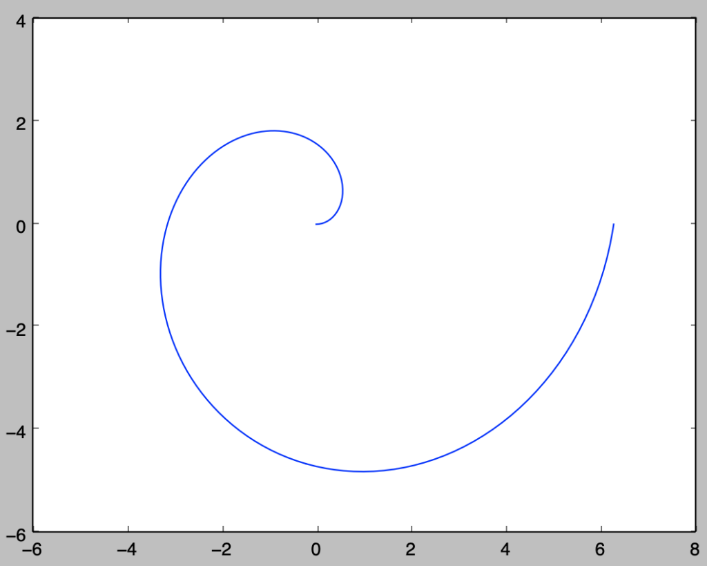
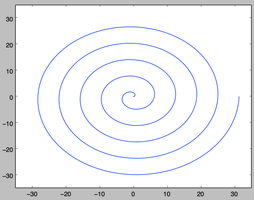
上図より、螺旋のような形状を描くことが確認できる。$\theta$を大きくした際の軌跡を確認するにあたって、以下ではさらに$0 \leq \theta \leq 10 \pi$の描画を行う。
a = 1.

theta = np.linspace(0,10*np.pi,1000)
r = a*theta

x = r*np.cos(theta)
y = r*np.sin(theta)

plt.ficure(7,7)
plt.plot(x,y)
plt.xlim([-35.,35.])
plt.ylim([-35.,35.])
plt.show()
・実行結果