$0^{\circ}$〜$360^{\circ}$や$0$〜$2 \pi$のように表される角度は周期を持ちますが、平均などを計算する際に周期を考慮する必要が生じます。当記事では角度の平均の計算にあたって三角関数を導入した計算の流れを確認し、直感的な理解ができるようにPythonを用いたプログラムを元に確認を行います。
当記事は「パターン認識と機械学習」の$2.3.8$節の「Periodic variables」を参考に作成を行いました。
また、$(o.xx)$の形式の式番号は「パターン認識と機械学習」の式番号に対応させました。
三角関数を用いた角度の平均の計算の流れ
$\theta_{i} \in [0,2 \pi]$の$\theta_{1}, \cdots \theta_{n}$が観測されたとき、平均の$\overline{\theta}$を計算を行うことを考える。
計算にあたっては、$\theta_{i}$を元に下記のように$x_{i},y_{i}$を定める。
$$
\large
\begin{align}
x_{i} &= r \cos{\theta_{i}} \\
y_{i} &= r \sin{\theta_{i}}
\end{align}
$$
上記では半径を$r$とおいたが、単位円を考えて$r=1$とおいても良い。このとき、$x_{i},y_{i}$の平均$\bar{x},\bar{y}$はそれぞれ下記のように計算できる。
$$
\large
\begin{align}
\bar{x} &= \sum_{i=1}^{n} x_{i} \\
&= \sum_{i=1}^{n} r \cos{\theta_{i}} \\
&= r \sum_{i=1}^{n} \cos{\theta_{i}} \\
\bar{y} &= \sum_{i=1}^{n} y_{i} \\
&= \sum_{i=1}^{n} r \sin{\theta_{i}} \\
&= r \sum_{i=1}^{n} \sin{\theta_{i}}
\end{align}
$$
ここで上記で計算を行った$\bar{x},\bar{y}$のなす角を$\overline{\theta}$と定めると、$\overline{\theta}$に関して下記が成立する。
$$
\large
\begin{align}
\tan{\overline{\theta}} &= \frac{\bar{y}}{\bar{x}} \\
&= \frac{\displaystyle \cancel{r} \sum_{i=1}^{n} \sin{\theta_{i}}}{\displaystyle \cancel{r} \sum_{i=1}^{n} \cos{\theta_{i}}} \\
&= \frac{\displaystyle \sum_{i=1}^{n} \sin{\theta_{i}}}{\displaystyle \sum_{i=1}^{n} \cos{\theta_{i}}} \\
\overline{\theta} &= \tan^{-1} \left[ \frac{\displaystyle \sum_{i=1}^{n} \sin{\theta_{i}}}{\displaystyle \sum_{i=1}^{n} \cos{\theta_{i}}} \right] \quad (2.169)
\end{align}
$$
Pythonを用いた角度の平均の計算
以下ではいくつかの例に対して、角度の平均の計算と図式化を行う。
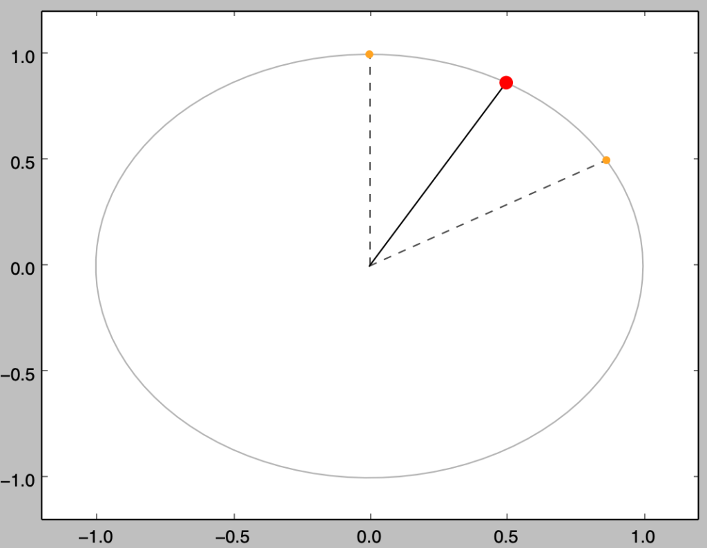
実行例①
$$
\large
\begin{align}
\theta_{1} &= \frac{1}{6} \pi \\
\theta_{2} &= \frac{1}{2} \pi
\end{align}
$$
上記の$\theta_{1}, \theta_{2}$の平均$\overline{\theta}$の計算は下記を実行することで行える。
import numpy as np
import matplotlib.pyplot as plt

r = 1
theta = np.array([np.pi/6., np.pi/2.])
x, y = np.cos(theta), np.sin(theta)

x_mean = np.mean(x)
y_mean = np.mean(y)
theta_mean = np.arctan(y_mean/x_mean)

theta_ = np.linspace(0.,2.*np.pi,100)
x_, y_ = np.cos(theta_), np.sin(theta_)

plt.plot(x_,y_,"k-",alpha=0.3,zorder=0)
plt.plot([0., x[0]],[0., y[0]],"k--",alpha=0.7,zorder=1), plt.plot([0., x[1]],[0., y[1]],"k--",alpha=0.7,zorder=1)
plt.plot([0., np.cos(theta_mean)],[0., np.sin(theta_mean)],"k-",alpha=1.0,zorder=1)
plt.scatter(x,y,color="orange",zorder=2)
plt.scatter(np.cos(theta_mean),np.sin(theta_mean),color="red",s=70,zorder=2)

plt.xlim([-1.2,1.2]), plt.ylim([-1.2,1.2])
plt.show()
・実行結果
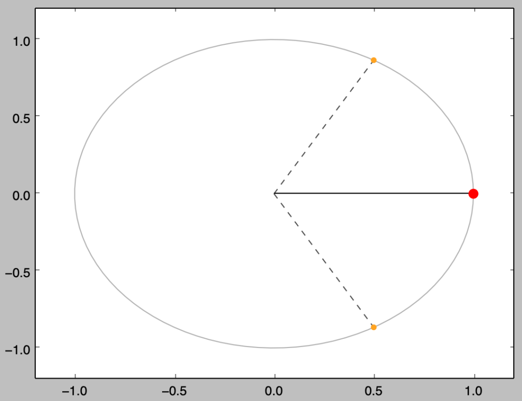
実行例②
$$
\large
\begin{align}
\theta_{1} &= \frac{1}{3} \pi \\
\theta_{2} &= \frac{5}{3} \pi
\end{align}
$$
上記の$\theta_{1}, \theta_{2}$の平均$\overline{\theta}$の計算は下記を実行することで行える。
r = 1
theta = np.array([np.pi/3., 5.*np.pi/3.])
x, y = np.cos(theta), np.sin(theta)

x_mean = np.mean(x)
y_mean = np.mean(y)
theta_mean = np.arctan(y_mean/x_mean)

theta_ = np.linspace(0.,2.*np.pi,100)
x_, y_ = np.cos(theta_), np.sin(theta_)

plt.plot(x_,y_,"k-",alpha=0.3,zorder=0)
plt.plot([0., x[0]],[0., y[0]],"k--",alpha=0.7,zorder=1), plt.plot([0., x[1]],[0., y[1]],"k--",alpha=0.7,zorder=1)
plt.plot([0., np.cos(theta_mean)],[0., np.sin(theta_mean)],"k-",alpha=1.0,zorder=1)
plt.scatter(x,y,color="orange",zorder=2)
plt.scatter(np.cos(theta_mean),np.sin(theta_mean),color="red",s=70,zorder=2)

plt.xlim([-1.2,1.2]), plt.ylim([-1.2,1.2])
plt.show()
・実行結果