

当記事は「基礎統計学Ⅲ 自然科学の統計学(東京大学出版会)」の読解サポートにあたってChapter.$2$の「線形モデルと最小二乗法」の章末問題の解説について行います。
基本的には書籍の購入者向けの解答例・解説なので、まだ入手されていない方は下記より入手をご検討ください。また、解説はあくまでサイト運営者が独自に作成したものであり、書籍の公式ページではないことにご注意ください。
https://www.amazon.co.jp/dp/4130420674
Contents
章末の演習問題について
問題2.1の解答例
i)
$[0,1]$の一様乱数に関してはNumPyのrandom.randを用いて$y_i$の生成を行う。
import numpy as np

np.random.seed(0)
u = np.random.rand(10,12)
epsilon = np.sum(u,axis=1)-6.
y = 15. + epsilon

print(y)
・実行結果
> print(y)
[ 16.47828279  16.17259914  14.48252679  15.08570806  13.76567862
  13.92641329  13.66679521  14.26112406  15.07466738  16.7132275 ]
ⅱ)
下記を実行することで$y_{ij}, i=1,2,…,5, j=1,2,…,5$の生成を行う。
import numpy as np

np.random.seed(0)
u = np.random.rand(5,5,12)
epsilon = np.sum(u,axis=2)-6.
y = np.array([np.repeat(2.,5), np.repeat(4.,5), np.repeat(6.,5), np.repeat(8.,5), np.repeat(10.,5)]) + epsilon

print(y)
・実行結果
> print(y)
[[  3.47828279   3.17259914   1.48252679   2.08570806   0.76567862]
 [  2.92641329   2.66679521   3.26112406   4.07466738   5.7132275 ]
 [  6.17470405   6.49753858   7.01033545   6.79519637   4.72282185]
 [  7.92514854   6.90028678   7.57093465   8.73749154   7.02365745]
 [  9.42140393  10.17896516  11.20754253  10.97396766  10.28374057]]
ⅲ)
下記を実行することで$y_i$の生成を行う。
import numpy as np

np.random.seed(0)
u = np.random.rand(10,12)
x = np.arange(1.,11.,1)
epsilon = np.sum(u,axis=1)-6.
y = 10-5*x+2*x**2+epsilon

print(y)
・実行結果
> print(y)
[   8.47828279    9.17259914   12.48252679   22.08570806   33.76567862
   50.92641329   71.66679521   97.26112406  127.07466738  161.7132275 ]
問題2.2の解答例
数式よりもNumPy形式の方が取り扱いやすいので、以下NumPy形式で表す。
i)
下記を実行することで$\mathbf{X}, \mathbf{X}^{T}\mathbf{X}, \mathbf{X}^{T}\mathbf{y}$を表すことができる。
import numpy as np

X = np.ones([10,1])
y = np.array([16.47828279, 16.17259914, 14.48252679, 15.08570806, 13.76567862, 13.92641329, 13.66679521, 14.26112406, 15.07466738, 16.7132275]).reshape([10,1])

print(X)
print(np.dot(X.T,X))
print(np.dot(X.T,y))
・実行結果
> print(X)
[[ 1.]
 [ 1.]
 [ 1.]
 [ 1.]
 [ 1.]
 [ 1.]
 [ 1.]
 [ 1.]
 [ 1.]
 [ 1.]]
> print(np.dot(X.T,X))
[[ 10.]]
> print(np.dot(X.T,y))
[[ 149.62702284]]
ⅱ)
下記を実行することで$\mathbf{X}, \mathbf{X}^{T}\mathbf{X}, \mathbf{X}^{T}\mathbf{y}$を表すことができる。
import numpy as np

X = np.zeros([25,6])
X[:,0] = 1.
X[0:5,1] = 1.
X[5:10,2] = 1.
X[10:15,3] = 1.
X[15:20,4] = 1.
X[20:25,5] = 1.
y = np.array([[3.47828279, 3.17259914, 1.48252679, 2.08570806, 0.76567862], [  2.92641329, 2.66679521, 3.26112406, 4.07466738, 5.7132275], [6.17470405, 6.49753858, 7.01033545, 6.79519637, 4.72282185], [7.92514854, 6.90028678, 7.57093465, 8.73749154, 7.02365745], [9.42140393, 10.17896516, 11.20754253, 10.97396766, 10.28374057]]).reshape([25,1])

print(X)
print(np.dot(X.T,X))
print(np.dot(X.T,y))
・実行結果
> print(X)
[[ 1.  1.  0.  0.  0.  0.]
 [ 1.  1.  0.  0.  0.  0.]
 [ 1.  1.  0.  0.  0.  0.]
...
 [ 1.  0.  0.  0.  0.  1.]
 [ 1.  0.  0.  0.  0.  1.]
 [ 1.  0.  0.  0.  0.  1.]
 [ 1.  0.  0.  0.  0.  1.]]
> print(np.dot(X.T,X))
[[ 25.   5.   5.   5.   5.   5.]
 [  5.   5.   0.   0.   0.   0.]
 [  5.   0.   5.   0.   0.   0.]
 [  5.   0.   0.   5.   0.   0.]
 [  5.   0.   0.   0.   5.   0.]
 [  5.   0.   0.   0.   0.   5.]]
> print(np.dot(X.T,y))
[[ 151.05075795]
 [  10.9847954 ]
 [  18.64222744]
 [  31.2005963 ]
 [  38.15751896]
 [  52.06561985]]
ⅲ)
下記を実行することで$\mathbf{X}, \mathbf{X}^{T}\mathbf{X}, \mathbf{X}^{T}\mathbf{y}$を表すことができる。
import numpy as np

X = np.ones([10,3])
X[:,1] = np.arange(1.,11.,1)
X[:,2] = X[:,1]**2
y = np.array([8.47828279, 9.17259914, 12.48252679, 22.08570806, 33.76567862, 50.92641329, 71.66679521, 97.26112406, 127.07466738, 161.7132275]).reshape([10,1])

print(X)
print(np.dot(X.T,X))
print(np.dot(X.T,y))
・実行結果
> print(X)
[[   1.    1.    1.]
 [   1.    2.    4.]
 [   1.    3.    9.]
 [   1.    4.   16.]
 [   1.    5.   25.]
 [   1.    6.   36.]
 [   1.    7.   49.]
 [   1.    8.   64.]
 [   1.    9.   81.]
 [   1.   10.  100.]]
> print(np.dot(X.T,X))
[[  1.00000000e+01   5.50000000e+01   3.85000000e+02]
 [  5.50000000e+01   3.85000000e+02   3.02500000e+03]
 [  3.85000000e+02   3.02500000e+03   2.53330000e+04]]
> print(np.dot(X.T,y))
[[   594.62702284]
 [  4667.56160689]
 [ 39389.13130627]]
問題2.3の解答例
scipy.linalg.invを用いて逆行列の計算を行う。
i)
import numpy as np
from scipy import linalg

X = np.ones([10,1])
y = np.array([16.47828279, 16.17259914, 14.48252679, 15.08570806, 13.76567862, 13.92641329, 13.66679521, 14.26112406, 15.07466738, 16.7132275]).reshape([10,1])
X_ = linalg.inv(np.dot(X.T,X))
theta = np.dot(X_,np.dot(X.T,y))

print(theta)
・実行結果
> print(theta)
[[ 14.96270228]]
ⅱ)
省略
ⅲ)
import numpy as np
from scipy import linalg

X = np.ones([10,3])
X[:,1] = np.arange(1.,11.,1)
X[:,2] = X[:,1]**2
y = np.array([8.47828279, 9.17259914, 12.48252679, 22.08570806, 33.76567862, 50.92641329, 71.66679521, 97.26112406, 127.07466738, 161.7132275]).reshape([10,1])
X_ = linalg.inv(np.dot(X.T,X))
theta = np.dot(X_,np.dot(X.T,y))

print(theta)
・実行結果
> print(theta)
[[ 13.31134241]
 [ -6.56004997]
 [  2.13588662]]
問題2.4の解答例
・備考
少々問題文の意図がわかりにくい印象だったので、ⅱ)の答えを先に確認した後に取り組む方が良いと思います。
i)
下記を実行することでそれぞれ計算を行うことができる。
import numpy as np

x, y = np.zeros([11,4]), np.zeros([11,4])
x[:,0], x[:,1], x[:,2] = np.array([10., 8., 13., 9., 11., 14., 6., 4., 12., 7., 5.]), np.array([10., 8., 13., 9., 11., 14., 6., 4., 12., 7., 5.]), np.array([10., 8., 13., 9., 11., 14., 6., 4., 12., 7., 5.])
x[:,3] = np.array([8., 8., 8., 8., 8., 8., 8., 19., 8., 8., 8.])
y[:,0] = np.array([8.04, 6.95, 7.58, 8.81, 8.33, 9.96, 7.24, 4.26, 10.84, 4.82, 5.68])
y[:,1] = np.array([9.14, 8.14, 8.74, 8.77, 9.26, 8.1, 6.13, 3.1, 9.13, 7.26, 4.74])
y[:,2] = np.array([7.46, 6.77, 12.74, 7.11, 7.81, 8.84, 6.08, 5.39, 8.15, 6.42, 5.73])
y[:,3] = np.array([6.58, 5.76, 7.71, 8.84, 8.47, 7.04, 5.25, 12.5, 5.56, 7.91, 6.89])

s_x, s_y, s_xy = np.sum((x-np.mean(x))**2, axis=0)/(x.shape[0]-1), np.sum((y-np.mean(y))**2, axis=0)/(x.shape[0]-1), np.sum((x-np.mean(x))*(y-np.mean(y)), axis=0)/(x.shape[0]-1)
r = s_xy/np.sqrt(s_x*s_y)

beta = np.zeros([4,2])
beta[:,1] = s_xy/s_x
beta[:,0] = np.mean(y)-beta[:,1]*np.mean(x,axis=0)

S_xx = np.sum((x-np.mean(x))**2, axis=0)
S_xy = np.sum((x-np.mean(x))*(y-np.mean(y)), axis=0)

e = y[:,0]-(beta[0,0]+beta[0,1]*x[:,0])
s_beta = np.sqrt(np.sum(e**2)/((x.shape[0]-2)*np.sum((x[:,0]-np.mean(x,axis=0)[0])**2)))
t = (beta[0,1]-0.)/s_beta

print("a. n: {}".format(x.shape[0]))
print("b. mean_x: {:.1f}".format(np.mean(x,axis=0)[0]))
print("c. mean_y: {:.1f}".format(np.mean(y,axis=0)[0]))
print("d. mean_y: {:.3f}".format(r[0]))
print("e. estimated beta_1: {:.1f}".format(beta[0,1]))
print("f. linear func: y = {:.0f} + {:.1f}x".format(beta[0,0],beta[0,1]))
print("g. S_xx: {:.1f}".format(S_xx[0]))
print("h. S_xy: {:.2f}".format(S_xy[0]))
print("i. {:.2f}".format(S_xy**2/S_xx))
print("j. t: {:.2f}".format(t))
・実行結果
a. n: 11
b. mean_x: 9.0
c. mean_y: 7.5
d. mean_y: 0.816
e. estimated beta_1: 0.5
f. linear func: y = 3 + 0.5x
g. S_xx: 110.0
h. S_xy: 54.99
i. 27.49
j. t: 4.24
なお、結果は巻末の解答に合わせて$(x_1,y_1)$に関するもののみを出力したが、それぞれの変数には他の値も格納した。どの$(x_i,y_i)$の組に対しても$(x_1,y_1)$と同様の結果が得られることは抑えておくと良い。
ⅱ)
import numpy as np
import matplotlib.pyplot as plt

x, y = np.zeros([11,4]), np.zeros([11,4])
x[:,0], x[:,1], x[:,2] = np.array([10., 8., 13., 9., 11., 14., 6., 4., 12., 7., 5.]), np.array([10., 8., 13., 9., 11., 14., 6., 4., 12., 7., 5.]), np.array([10., 8., 13., 9., 11., 14., 6., 4., 12., 7., 5.])
x[:,3] = np.array([8., 8., 8., 8., 8., 8., 8., 19., 8., 8., 8.])
y[:,0] = np.array([8.04, 6.95, 7.58, 8.81, 8.33, 9.96, 7.24, 4.26, 10.84, 4.82, 5.68])
y[:,1] = np.array([9.14, 8.14, 8.74, 8.77, 9.26, 8.1, 6.13, 3.1, 9.13, 7.26, 4.74])
y[:,2] = np.array([7.46, 6.77, 12.74, 7.11, 7.81, 8.84, 6.08, 5.39, 8.15, 6.42, 5.73])
y[:,3] = np.array([6.58, 5.76, 7.71, 8.84, 8.47, 7.04, 5.25, 12.5, 5.56, 7.91, 6.89])

for i in range(x.shape[1]):
    plt.subplot(2,2,i)
    plt.scatter(x[:,i],y[:,i],color="green")
    plt.plot(x[:,i],beta[0]+beta[1]*x[:,i],color="limegreen")

plt.show()
・実行結果
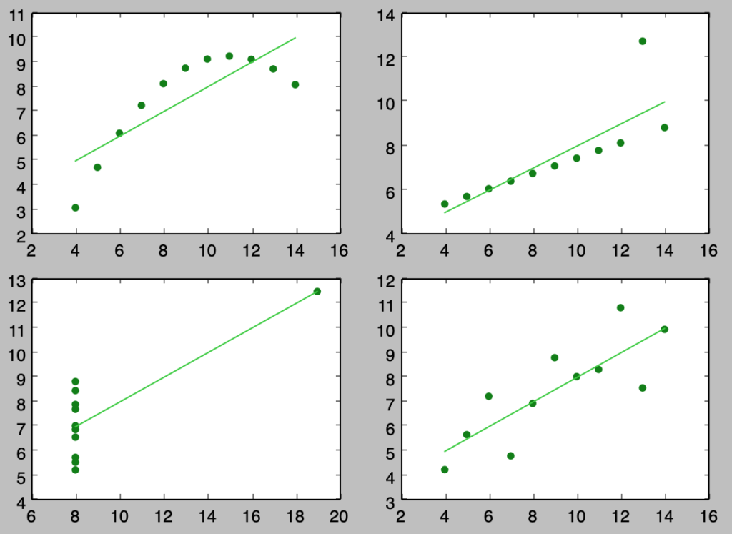
上記のように散布図を描くことで、全く異なる分布であるにも関わらず同じ係数が推定される場合があることに注意が必要であることがわかる。
問題2.5の解答例
問題2.6の解答例
下記を実行することで回帰係数の推定と、散布図や回帰式の図示を行うことができる。
import numpy as np
import matplotlib.pyplot as plt

x = np.array([8., 6., 11., 22., 14., 17., 18., 24., 19., 23., 26., 40.])
y = np.array([59., 58., 56., 53., 50., 45., 43., 42., 39., 38., 30., 27.])

beta = np.zeros(2)
beta[1] = np.sum((x-np.mean(x))*(y-np.mean(y)))/np.sum((x-np.mean(x))**2)
beta[0] = np.mean(y)-beta[1]*np.mean(x)

print("beta_0: {:.3f}".format(beta[0]))
print("beta_1: {:.3f}".format(beta[1]))

plt.scatter(x,y,color="green")
plt.plot(x,beta[0]+beta[1]*x,color="limegreen")
plt.show()
・実行結果
> plt.scatter(x,y,color="green")
beta_0: 64.247
> print("beta_1: {:.3f}".format(beta[1]))
beta_1: -1.013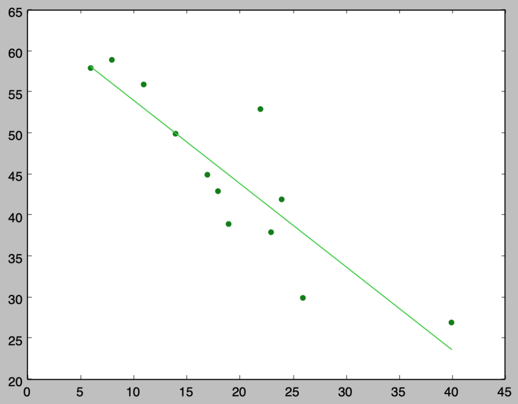
また、下記を実行することで帰無仮説$H_0: \beta_1=0$に関する検定を行うことができる。
import numpy as np
from scipy import stats

x = np.array([8., 6., 11., 22., 14., 17., 18., 24., 19., 23., 26., 40.])
y = np.array([59., 58., 56., 53., 50., 45., 43., 42., 39., 38., 30., 27.])

beta = np.zeros(2)
beta[1] = np.sum((x-np.mean(x))*(y-np.mean(y)))/np.sum((x-np.mean(x))**2)
beta[0] = np.mean(y)-beta[1]*np.mean(x)

e = y-(beta[0]+beta[1]*x)
s_e = np.sqrt(np.sum(e**2)/(x.shape[0]-2))
s_beta = s_e/np.sqrt(np.sum((x-np.mean(x))**2))

t = (beta[1]-0)/s_beta

if np.abs(t) > stats.t.ppf(1.-0.025,x.shape[0]-2):
    print("t: {:.2f}, reject H_0.".format(t))
else:
    print("t: {:.2f}, accept H_0.".format(t))
・実行結果
t: -5.88, reject H_0.問題2.7の解答例
i)
P.45の議論を元に導出を行う。
$x$の平均を$\bar{x}$、$y$の平均を$\bar{y}$、$\displaystyle S_{xx}=\sum_{i=1}^{15} (x_i-\bar{x})^2$、$\displaystyle S_{xy}=\sum_{i=1}^{15} (x_i-\bar{x})(y_i-\bar{y})$とする。このとき、それぞれの値は下記のように計算できる。
$$
\large
\begin{align}
\bar{x} &= \frac{1}{15}(7.2+4.8+5.2+4.9+5.4+6.4+6.8+8.0 \\
&+6.0+6.7+7.0+8.0+7.3+4.6+4.2) \\
&= 6.1666… \\
\bar{y} &= \frac{1}{15}(8.4+5.4+6.3+6.8+8.0+11.1+12.3+13.3 \\
&+8.4+9.5+10.4+12.7+10.3+7.0+5.1) \\
&= 9.0 \\
S_{xx} &= (7.2-6.167)^2+… \\
&= 21.853 \\
S_{xy} &=(7.2-6.167)(8.4-9.0)+… \\
&= 41.520
\end{align}
$$
このとき下記が成立する。
$$
\large
\begin{align}
y &= \bar{y}+\frac{S_{xy}}{S_{xx}}(x-\bar{x}) \\
&= 9+\frac{21.853}{41.520}(x-6.167) \\
&= 1.9x-2.716
\end{align}
$$
上記より、$\beta_{0}=-2.716$、$\beta_{1}=1.9$が成立する。
ⅱ)
i)で求めた$y=1.9x-2.716$に$x=6.9$を代入する。
$$
\large
\begin{align}
y &= 1.9x-2.716 \\
&= 1.9 \times 6.9 – 2.716 \\
&= 10.39
\end{align}
$$
ⅲ)
下記を実行することで計算を行うことができる。
import numpy as np
from scipy import stats

x = np.array([7.2, 4.8, 5.2, 4.9, 5.4, 6.4, 6.8, 8.0, 6.0, 6.7, 7.0, 8.0, 7.3, 4.6, 4.2])
y = np.array([8.4, 5.4, 6.3, 6.8, 8.0, 11.1, 12.3, 13.3, 8.4, 9.5, 10.4, 12.7, 10.3, 7.0, 5.1])

s_x = np.sum((x-np.mean(x))**2)
s_xy = np.sum((x-np.mean(x))*(y-np.mean(y)))

beta = np.zeros(2)
beta[1] = s_xy/s_x
beta[0] = np.mean(y)-beta[1]*np.mean(x)

expected_y = beta[0] + beta[1]*6.9

sigma2 = (np.sum(y**2)-np.sum(y)**2/x.shape[0]-s_xy**2/s_x)/(x.shape[0]-2)
y_range = np.sqrt((1./x.shape[0]+(6.9-np.mean(x))/s_x)*sigma2)

interval_y = np.array([expected_y+stats.t.ppf(0.025,x.shape[0]-2)*y_range, expected_y+stats.t.ppf(0.975,x.shape[0]-2)*y_range])

print(interval_y)
・実行結果
> print(interval_y)
array([  9.57708628,  11.2094909 ])
iv)
下記を実行することで$H_0: \beta_1=2$の検定を行うことができる。
import numpy as np
from scipy import stats

x = np.array([7.2, 4.8, 5.2, 4.9, 5.4, 6.4, 6.8, 8.0, 6.0, 6.7, 7.0, 8.0, 7.3, 4.6, 4.2])
y = np.array([8.4, 5.4, 6.3, 6.8, 8.0, 11.1, 12.3, 13.3, 8.4, 9.5, 10.4, 12.7, 10.3, 7.0, 5.1])

beta = np.zeros(2)
beta[1] = np.sum((x-np.mean(x))*(y-np.mean(y)))/np.sum((x-np.mean(x))**2)
beta[0] = np.mean(y)-beta[1]*np.mean(x)

expected_y = beta[0] + beta[1]*6.9

e = y - (beta[0]+beta[1]*x)
s_error = np.sqrt(np.sum(e**2)/(x.shape[0]-2))
s_error_beta = s_error/np.sqrt(np.sum((x-np.mean(x))**2))

t = (beta[1]-2.)/s_error_beta
if np.abs(t)>stats.t.ppf(1.-0.025,x.shape[0]-2):
    print("t: {:.3f}, reject H_0".format(t))
else:
    print("t: {:.3f}, accept H_0".format(t))
・実行結果
t: -0.392, accept H_0問題2.8の解答例
問題2.9の解答例
問題2.10の解答例
i)
誤差項$\epsilon_i$に関して、二乗和を考えると下記のように表すことができる。
$$
\large
\begin{align}
\sum_{i=1}^{n} \epsilon_i^2 = \sum_{i=1}^{n} (y_i – \beta x_i)^2
\end{align}
$$
上記を$\beta$で偏微分し、正規方程式を考え、下記のように$\beta$に関して解く。
$$
\large
\begin{align}
\frac{\partial}{\partial \beta} \sum_{i=1}^{n} (y_i – \beta x_i)^2 &= 0 \\
-2 \sum_{i=1}^{n} (y_i – \beta x_i) x_i &= 0 \\
\sum_{i=1}^{n} x_i y_i &= \beta \sum_{i=1}^{n} x_i^2 \\
\beta \sum_{i=1}^{n} x_i^2 &= \sum_{i=1}^{n} x_i y_i \\
\beta &= \frac{\sum_{i=1}^{n} x_i y_i}{\sum_{i=1}^{n} x_i^2}
\end{align}
$$
よって$\beta$の最小二乗推定量$\hat{\beta}$は下記のように表すことができる。
$$
\large
\begin{align}
\hat{\beta} = \frac{\sum_{i=1}^{n} x_i y_i}{\sum_{i=1}^{n} x_i^2}
\end{align}
$$