当記事は「統計検定$2$級対応 統計学基礎(東京図書)」の読解サポートにあたって第$1$章の「データの記述と要約」に関して演習問題を中心に解説を行います。平均、分散、標準偏差、相関係数、回帰などを考える記述統計は統計学の実用にあたってよく用いられるので、演習を通して抑えておくと良いと思います。
本章のまとめ
練習問題解説
問$1$.$1$
問$1$.$2$
それぞれの計算を行うにあたってPythonを用いる。変数に関しては共通で用いるので、重複部分は省略を行った。
import numpy as np
import matplotlib.pyplot as plt

x1 = np.array([30., 30., 40., 40., 50., 50., 60., 60., 70., 70.])
x2 = np.array([45., 60., 50., 65., 70., 50., 55., 60., 70., 75.])

mean_x1 = np.mean(x1)
mean_x2 = np.mean(x2)
・$[1]$
下記を実行することで平均と標準偏差の計算を行うことができる。
sd1 = np.sqrt(np.mean(x1**2)-mean_x1**2)
sd2 = np.sqrt(np.mean(x2**2)-mean_x2**2)

print("Test1. mean: {:.1f}, sd: {:.2f}".format(mean_x1,sd1))
print("Test2. mean: {:.1f}, sd: {:.2f}".format(mean_x2,sd2))
実行結果
Test1. mean: 50.0, sd: 14.14
Test2. mean: 60.0, sd: 9.49
・$[2]$
$C$さんの標準化得点は下記のように計算できる。
z_c1 = (x1[2]-mean_x1)/sd1
z_c2 = (x2[2]-mean_x2)/sd2

print("z_c1: {:.2f}".format(z_c1))
print("z_c2: {:.2f}".format(z_c2))
実行結果
z_c1: -0.71
z_c2: -1.05
・$[3]$
下記を実行することで変動係数を計算できる。
print("CV1: {:.2f}".format(sd1/mean_x1))
print("CV2: {:.2f}".format(sd2/mean_x2))
実行結果
CV1: 0.28
CV2: 0.16
・$[4]$
下記を実行することで散布図の描画を行える。
plt.scatter(x1,x2)
plt.show()
実行結果
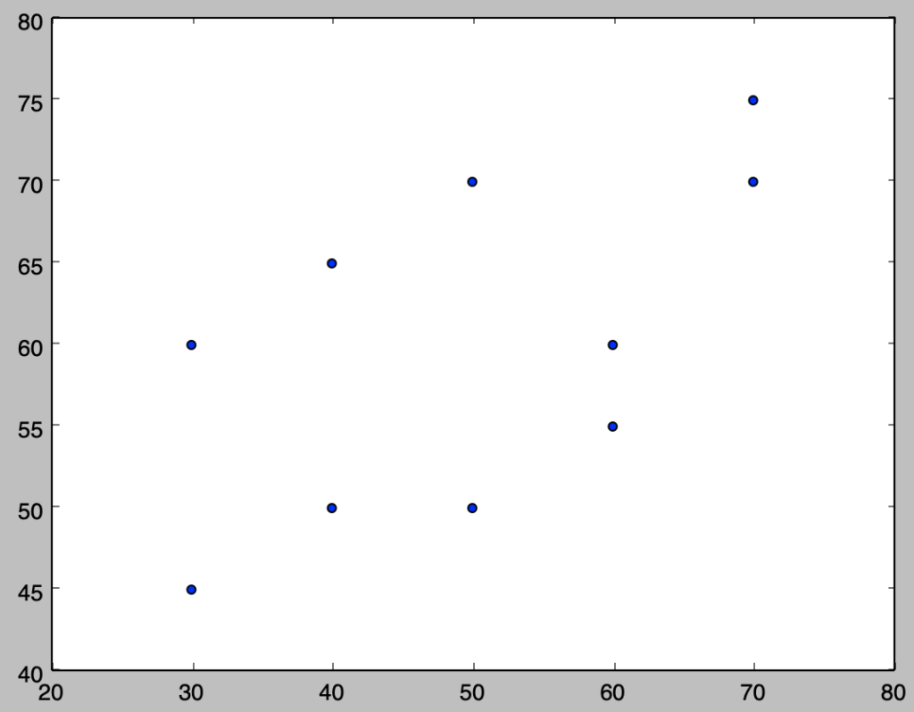
また、相関係数は下記を実行することで計算できる。
cov_x12 = np.mean(x1*x2)-mean_x1*mean_x2
r = cov_x12/(sd1*sd2)
print("r: {:.2f}".format(r))
実行結果
r: 0.60・$[5]$
下記を計算することで$y_i=ax_i+b$の係数$a, b$を計算できる。
a = cov_x12/sd1**2
b = mean_x2 - a*mean_x1
print("a: {:.2f}, b: {:.2f}".format(a,b))
実行結果
a: 0.40, b: 40.00・$[6]$
下記を実行することで計算できる。
print("R^2: {:2f}".format(r**2))実行結果
R^2: 0.36問$1$.$3$
・$[1]$
下記のような計算を行うことでそれぞれ計算できる。
import numpy as np

x = np.array([0.39, 0.72, 1., 1.52, 5.2, 9.54, 19.19, 30.07])
y = np.array([0.24, 0.62, 1., 1.88, 11.86, 29.46, 84.01, 164.79])

s_x_2 = np.mean((x-np.mean(x))**2)
s_y_2 = np.mean((y-np.mean(y))**2)
s_xy = np.mean((x-np.mean(x))*(y-np.mean(y)))

a = s_xy/s_x_2
b = np.mean(y) - a*np.mean(x)
r = s_xy / np.sqrt(s_x_2*s_y_2)

if b > 0:
    print("Estimated line: y={:.2f}x+{:.2f}".format(a,b))
else:
    print("Estimated: y={:.2f}x{:.2f}".format(a,b))
print("coef of determination: {:.2f}".format(r**2))
・実行結果
Estimated line: y=5.38x-8.79
coef of determination: 0.98
・$[2]$
下記のような計算を行うことでそれぞれ計算できる。
import numpy as np

x = np.array([0.39, 0.72, 1., 1.52, 5.2, 9.54, 19.19, 30.07])
x2 = x**2
y = np.array([0.24, 0.62, 1., 1.88, 11.86, 29.46, 84.01, 164.79])

s_x_2 = np.mean((x2-np.mean(x2))**2)
s_y_2 = np.mean((y-np.mean(y))**2)
s_xy = np.mean((x2-np.mean(x2))*(y-np.mean(y)))

a = s_xy/s_x_2
b = np.mean(y) - a*np.mean(x2)
r = s_xy / np.sqrt(s_x_2*s_y_2)

if b > 0:
    print("Estimated line: y={:.2f}x^2+{:.2f}".format(a,b))
else:
    print("Estimated: y={:.2f}x{:.2f}".format(a,b))
print("coef of determination: {:.2f}".format(r**2))
・実行結果
Estimated line: y=0.18x^2+4.80
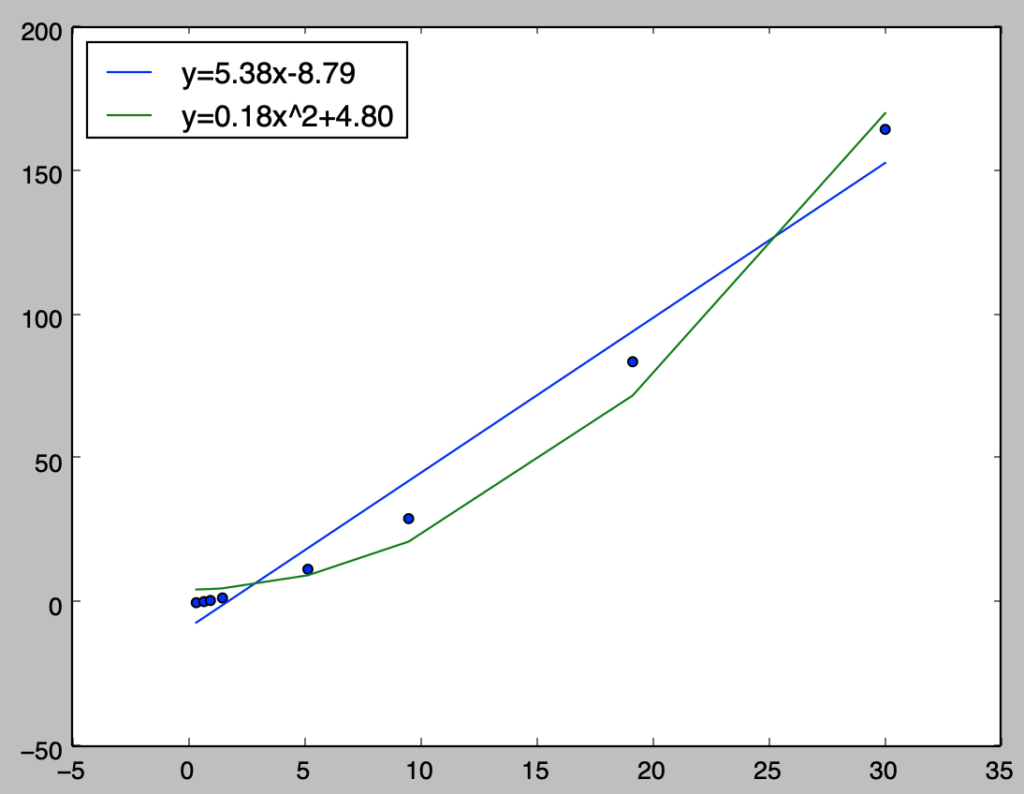
coef of determination: 0.99それぞれの結果は下記のように図示することができる。
import numpy as np
import matplotlib.pyplot as plt

x = np.array([0.39, 0.72, 1., 1.52, 5.2, 9.54, 19.19, 30.07])
x2 = x**2
y = np.array([0.24, 0.62, 1., 1.88, 11.86, 29.46, 84.01, 164.79])

s_x_2 = np.mean((x-np.mean(x))**2)
s_xy = np.mean((x-np.mean(x))*(y-np.mean(y)))
s_x_2_ = np.mean((x2-np.mean(x2))**2)
s_y_2 = np.mean((y-np.mean(y))**2)
s_xy_ = np.mean((x2-np.mean(x2))*(y-np.mean(y)))

a = s_xy/s_x_2
b = np.mean(y) - a*np.mean(x)
r = s_xy / np.sqrt(s_x_2*s_y_2)
a_ = s_xy_/s_x_2_
b_ = np.mean(y) - a_*np.mean(x2)
r_ = s_xy_ / np.sqrt(s_x_2_*s_y_2)

plt.scatter(x,y)
plt.plot(x,a*x+b,label="y=5.38x-8.79")
plt.plot(x,a_*x2+b_,label="y=0.18x^2+4.80")

plt.legend(loc="upper left")
plt.show()
・実行結果