
数式だけの解説ではわかりにくい場合もあると思われるので、統計学の手法や関連する概念をPythonのプログラミングで表現します。当記事では確率過程(stochastic process)の理解にあたって、ブラウン運動やポアソン過程のPythonでの実装を取り扱いました。
・Pythonを用いた統計学のプログラミングまとめ
https://www.hello-statisticians.com/stat_program
ブラウン運動
標準ブラウン運動・ウィーナー過程
標準ブラウン運動$N(0, t)$はウィーナー過程と呼ばれることもある。標準ブラウン運動は下記のように表現できる。
import numpy as np
import matplotlib.pyplot as plt
from scipy import stats

np.random.seed(0)

x = np.arange(0,100,1)
y = np.zeros([x.shape[0],5])

y[0,:] = stats.norm.rvs(size=5)
for i in range(x.shape[0]-1):
    y[i+1,:] = y[i,:] + stats.norm.rvs(size=5)

for i in range(y.shape[1]):
    plt.plot(x,y[:,i])

plt.show()
・実行結果
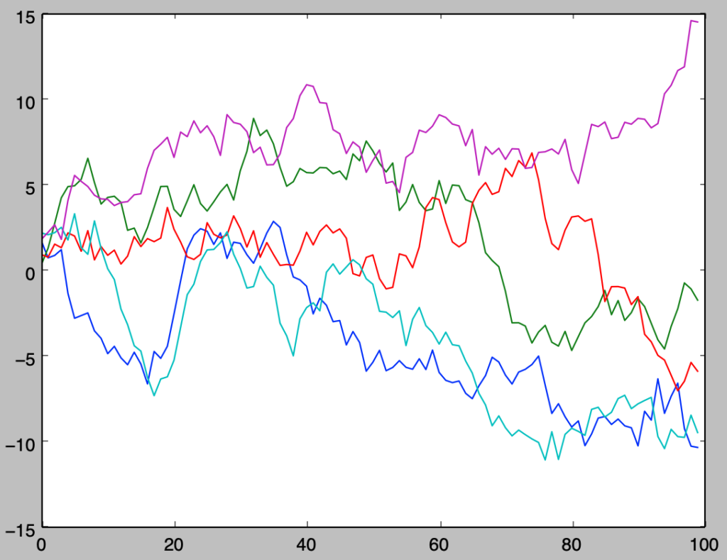
正規乱数の生成を簡易化するにあたってscipy.stats.norm.rvsを用いた。パッケージを用いない際は乗算合同法やM系列、メルセンヌツイスタ法などを用いて作成した一様乱数を元に中心極限定理の応用やボックス・ミュラー法を用いて生成することができる。
https://www.hello-statisticians.com/explain-terms-cat/random_sampling1.html
https://www.hello-statisticians.com/explain-books-cat/toukeigaku-aohon/stat_blue_ch11.html
ブラウン運動
確率過程の生成
下記を実行することでブラウン運動$N(\mu t, t)$を生成することができる。
import numpy as np
import matplotlib.pyplot as plt
from scipy import stats

np.random.seed(0)

mu, sigma = 0.2, 1
x = np.arange(0,100,1)
y = np.zeros([x.shape[0],5])

y[0,:] = stats.norm.rvs(size=5)
for i in range(x.shape[0]-1):
    y[i+1,:] = y[i,:] + stats.norm.rvs(mu,sigma,size=5)

for i in range(y.shape[1]):
    plt.plot(x,y[:,i])

plt.show()
・実行結果
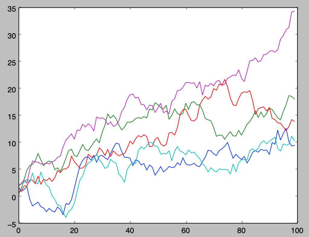
上記の生成にあたっては「標準ブラウン運動」と同じ乱数を用いたので、$\mu=0.2$に基づく増加のトレンド以外は類似の動きであることも確認できる。
確率過程のパラメータ推定
ブラウン運動$B_t \sim N(\mu t, \sigma^2 t)$に対して、$Z_k = B_{k \Delta}-B_{(k-1) \Delta} \sim N(\mu \Delta, \sigma^2 \Delta), k=1,2,…,n$とおくとき、$\mu, \sigma^2$の推定値$\hat{\mu}, \hat{\sigma^2}$は下記のように表せる。
$$
\large
\begin{align}
\hat{\mu} \Delta &= \frac{1}{n} \sum_{k=1}^{n} Z_k \\
\hat{\sigma}^2 \Delta + (\hat{\mu} \Delta)^2 &= \frac{1}{n} \sum_{k=1}^{n} Z_k^2
\end{align}
$$
パラメータ推定にあたって、最尤法・モーメント法のどちらを用いても上記の式が導出できる。上記を$\hat{\mu}, \hat{\sigma}^2$に関して解くと下記が得られる。
$$
\large
\begin{align}
\hat{\mu} &= \frac{1}{n \Delta} \sum_{k=1}^{n} Z_k \\
\hat{\sigma}^2 &= \frac{1}{n \Delta} \sum_{k=1}^{n} Z_k^2 – \hat{\mu}^2 \Delta
\end{align}
$$
ここまでの内容を元に前項で生成を行った確率過程のパラメータ推定を下記を実行することで行うことができる。
import numpy as np
import matplotlib.pyplot as plt
from scipy import stats

np.random.seed(0)

mu, sigma = 0.2, 1
x = np.arange(0,100,1)
y = np.zeros([x.shape[0],5])

y[0,:] = stats.norm.rvs(size=5)
for i in range(x.shape[0]-1):
    y[i+1,:] = y[i,:] + stats.norm.rvs(mu,sigma,size=5)

diff = y
diff[1:diff.shape[0],:] = diff[1:diff.shape[0],:] - diff[0:(diff.shape[0]-1),:]

mu_estimate = np.mean(diff, axis=0)
sigma2_estimate = np.mean(diff**2, axis=0) - mu_estimate**2

print("Estimated mu: {}".format(mu_estimate))
print("Estimated sigma^2: {}".format(sigma2_estimate))
・実行結果
> print("Estimated mu: {}".format(mu_estimate))
Estimated mu: [ 0.09504339  0.1811264   0.13958733  0.10372601  0.34374467]
> print("Estimated sigma^2: {}".format(sigma2_estimate))
Estimated sigma^2: [ 1.01006428  0.91386789  0.99829055  1.06096954  0.92964815]
サンプル数を$n=100$から$n=10,000$に増やし、推定値の変化を確認する。
np.random.seed(0)

mu, sigma = 0.2, 1
x = np.arange(0,10000,1)
y = np.zeros([x.shape[0],5])

y[0,:] = stats.norm.rvs(size=5)
for i in range(x.shape[0]-1):
    y[i+1,:] = y[i,:] + stats.norm.rvs(mu,sigma,size=5)

diff = y
diff[1:diff.shape[0],:] = diff[1:diff.shape[0],:] - diff[0:(diff.shape[0]-1),:]

mu_estimate = np.mean(diff, axis=0)
sigma2_estimate = np.mean(diff**2, axis=0) - mu_estimate**2

print("Estimated mu: {}".format(mu_estimate))
print("Estimated sigma^2: {}".format(sigma2_estimate))
・実行結果
> print("Estimated mu: {}".format(mu_estimate))
Estimated mu: [ 0.1966156   0.2103942   0.18599239  0.1893911   0.19853666]
> print("Estimated sigma^2: {}".format(sigma2_estimate))
Estimated sigma^2: [ 1.00373888  1.00122736  0.99122914  0.99615878  0.97360955]
サンプル数を$n=10,000$に設定すると、$\mu=0.2$周辺の推定値が確認でき、この推定値は概ね妥当であると考えることができる。
また、ここでは$\Delta=1$を元に考えたが、高頻度観測(high frequent observations)を行う際も$\Delta$の値を変えるだけで、同様に下記の式を適用し、パラメータ推定を行うことができることも抑えておくと良い。
$$
\large
\begin{align}
\hat{\mu} &= \frac{1}{n \Delta} \sum_{k=1}^{n} Z_k \\
\hat{\sigma}^2 &= \frac{1}{n \Delta} \sum_{k=1}^{n} Z_k^2 – \hat{\mu}^2 \Delta
\end{align}
$$
ポアソン過程
ポアソン過程の生成
下記を実行することでポアソン過程$Po(\lambda t)$を生成することができる。
import numpy as np
import matplotlib.pyplot as plt
from scipy import stats

np.random.seed(0)

lamb = 0.2
x = np.arange(0,100,1)
y = np.zeros([x.shape[0],3])

y[0,:] = stats.norm.rvs(size=3)
for i in range(x.shape[0]-1):
    y[i+1,:] = y[i,:] + stats.poisson.rvs(lamb,size=3)

x_ = np.repeat(x,2)
y_ = np.zeros([200,3])
for i in range(1,200):
    y_[i,:] = y[(i-1)//2,:]

for i in range(y.shape[1]):
    plt.plot(x_,y_[:,i])

plt.show()
・実行結果
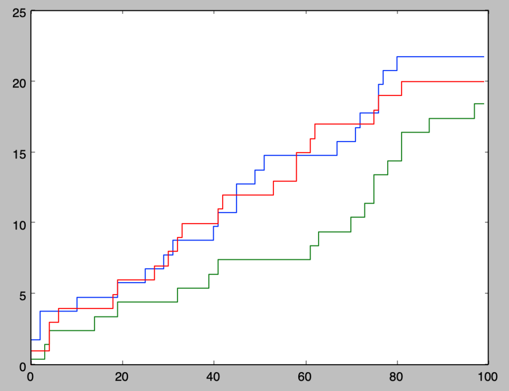
plot(x,y[:,i])をそのまま実行すると、階段状のグラフが表現できないので、x_とy_を作成し、描画を行った。
ポアソン過程のパラメータ推定
ポアソン過程$N_t \sim Po(\lambda t)$に対して、$M_k = N_{k \Delta}-N_{(k-1) \Delta} \sim Po(\lambda \Delta), k=1,2,…,n$とおくとき、$\lambda$の推定値$\hat{\lambda}$は下記のように表せる。
$$
\large
\begin{align}
\hat{\lambda} = \frac{1}{n \Delta} \sum_{k=1}^{n} M_k = \frac{N_{n \Delta}}{n \Delta}
\end{align}
$$
ここまでの内容を元に前項で生成を行った確率過程のパラメータ推定を下記を実行することで行うことができる。
import numpy as np
import matplotlib.pyplot as plt
from scipy import stats

np.random.seed(0)

lamb = 0.2
x = np.arange(0,100,1)
y = np.zeros([x.shape[0],3])

y[0,:] = stats.norm.rvs(size=3)
for i in range(x.shape[0]-1):
    y[i+1,:] = y[i,:] + stats.poisson.rvs(lamb,size=3)

diff = y
diff[1:diff.shape[0],:] = diff[1:diff.shape[0],:] - diff[0:(diff.shape[0]-1),:]

lambda_estimate = np.mean(diff, axis=0)

print("Estimated lambda: {}".format(lambda_estimate))
・実行結果
> print("Estimated lambda: {}".format(lambda_estimate))
Estimated lambda: [ 0.21764052  0.18400157  0.19978738]
サンプル数を$n=100$から$n=10,000$に増やし、推定値の変化を確認する。
np.random.seed(0)

lamb = 0.2
x = np.arange(0,10000,1)
y = np.zeros([x.shape[0],3])

y[0,:] = stats.norm.rvs(size=3)
for i in range(x.shape[0]-1):
    y[i+1,:] = y[i,:] + stats.poisson.rvs(lamb,size=3)

diff = y
diff[1:diff.shape[0],:] = diff[1:diff.shape[0],:] - diff[0:(diff.shape[0]-1),:]

lambda_estimate = np.mean(diff, axis=0)

print("Estimated lambda: {}".format(lambda_estimate))
・実行結果
> print("Estimated lambda: {}".format(lambda_estimate))
Estimated lambda: [ 0.20237641  0.19824002  0.20289787]
サンプル数を$n=10,000$に設定すると、$\lambda=0.2$周辺の推定値が確認でき、この推定値は概ね妥当であると考えることができる。