
自動微分(Automatic Differentiation)は大規模なニューラルネットワークであるDeepLearningの学習における誤差逆伝播などに用いられる手法です。当記事では自動微分の仕組みとPythonを用いた基本的な実装方針について取りまとめました。
作成にあたっては「ゼロから作るDeep Learning」の第$5$章「誤差逆伝播法」の内容を主に参照しました。
・用語/公式解説
https://www.hello-statisticians.com/explain-terms
Contents
自動微分の仕組み
合成関数の微分
$y=f(u), u = g(x)$のとき合成関数$y=f(g(x))$の$x$に関する微分は下記のように得られる。
$$
\large
\begin{align}
\frac{dy}{dx} = \frac{dy}{du} \cdot \frac{du}{dx}
\end{align}
$$
上記の「合成関数の微分の公式」は「連鎖率(chain rule)」のようにいう場合もある。式の詳しい導出は下記で取り扱った。
数式微分・数値微分の活用における課題
計算機で微分を取り扱う際の手法は数式微分(Symbolic differenetiation)、数値微分(Numerical differenetiation)、自動微分(Automatic differenetiation)の$3$つに大別できる。
「数式微分」は数学的に導関数を計算し入力値を代入することで計算を行う手法、「数値微分」は$\displaystyle \frac{f(x+\Delta)-f(x)}{\Delta x}$に基づいて近似的に計算を行う手法である。ニューラルネットワークの誤差関数のような複雑な合成関数の微分を取り扱う場合、数式微分では導関数の導出が大変複雑になり、数値微分はパラメータ数が多い場合計算量が多くなる。このような解決にあたって用いられるのが自動微分である。
たとえば下記の演習ではロジスティック回帰の勾配の計算について取り扱ったが、途中式がなかなか複雑である。ニューラルネットワークはロジスティック回帰を複雑化したものであると見なすこともできるので、数式微分を用いると計算がさらに複雑になる。
自動微分の仕組み
前項の課題の解決にあたってニューラルネットワークの学習にあたって実用的に用いられるのが自動微分(Automatic Differentiation)である。自動微分は数式微分と同様に「合成関数の微分の公式」を用いるが、「中間変数の値を代入してから積を計算すること」によりスムーズに計算を行うことができる。
たとえば$f(x) = e^{x^{2}}$の$f'(1)$の値を計算するにあたって、数式微分と自動微分はそれぞれ下記のように値を計算する。
・数式微分
$u=x^{2}, y=e^{u}$とおき、下記のように$f'(x)$を計算する。
$$
\large
\begin{align}
f'(x) &= \frac{dy}{dx} = \frac{dy}{du} \cdot \frac{du}{dx} \\
&= e^{u} \cdot 2x \\
&= 2x e^{x^{2}}
\end{align}
$$
上記より$f'(1) = 2e^{1} = 2e$の値を計算する。
・自動微分
$u=x^{2}, y=e^{u}$とおき、下記のように$f'(x)$を計算する。
$$
\large
\begin{align}
f'(x) &= \frac{dy}{dx} = \frac{dy}{du} \cdot \frac{du}{dx} \\
&= e^{u} \cdot 2x
\end{align}
$$
$x=1$のとき$u=1$であるので、$f'(1) = e^{1} \cdot 2 = 2e$を計算する。
「数式微分」と「自動微分」は基本的には同じ公式に基づいて同様な計算を行うが、「数式微分」が「すべて$x$の式で表さなければいけない」一方で「自動微分」は「中間変数の$u$が得られれば計算が可能」である。
よって、中間変数の$u$の値を効率よく保持しておけるならば「自動微分」に基づいてシンプルに結果を計算することができる。
自動微分の基本的な実装方針
実装方針
基本的には「演算」をクラス化し、順伝播(forward propagation)と逆伝播(back propagation)を同じクラスで取り扱うことで逆伝播の計算の効率化を実現する。
乗算のクラス化
全容
乗算は下記のようにクラス化することができる。
class MulLayer:
    def __init__(self):
        self.x = None
        self.y = None

    def forward(self, x, y):
        self.x = x
        self.y = y
        out = x*y
        return out

    def backward(self, dout):
        dx = dout * self.y
        dy = dout * self.x
        return dx, dy
上記のクラスは下記のように用いることができる。
apple = 100.
apple_num = 2.
tax = 1.1

mul_apple_layer = MulLayer()
mul_tax_layer = MulLayer()

# forward
apple_price = mul_apple_layer.forward(apple, apple_num)
price = mul_tax_layer.forward(apple_price, tax)

print(price)

# backward
dprice = 1.
dapple_price, dtax = mul_tax_layer.backward(dprice)
dapple, dapple_num = mul_apple_layer.backward(dapple_price)

print(dapple_price, dtax)
print(dapple, dapple_num)
・実行結果
220.00000000000003
1.1 200.0
2.2 110.00000000000001
順伝播による計算
xとyの積の計算は下記のようにforwardメソッドで実装される。
class MulLayer:
    〜省略〜

    def forward(self, x, y):
        self.x = x
        self.y = y
        out = x*y
        return out

    〜省略〜
out = x*yでoutを計算しreturnで出力するのと同時にself.x = xとself.y = yによって入力変数をインスタンスに保持させることを抑えておくと良い。
逆伝播による勾配の取得
xとyの積の計算は下記のようにforwardメソッドで実装される。
class MulLayer:
    〜省略〜

    def backward(self, dout):
        dx = dout * self.y
        dy = dout * self.x
return dx, dyxyを$x$について偏微分すると$y$、$y$について偏微分すると$x$、が得られることからdx = dout * self.yとdy = dout * self.xの処理を理解すると良い。
加算のクラス化
全容
class AddLayer:
    def __init__(self):
        pass

    def forward(self, x, y):
        out = x+y
        return out

    def backward(self, dout):
        dx = dout*1
        dy = dout*1
        return dx, dy
上記のクラスは下記のように用いることができる。
apple = 100.
apple_num = 2.
orange = 150.
orange_num = 3.
tax = 1.1

mul_apple_layer = MulLayer()
mul_orange_layer = MulLayer()
add_apple_orange_layer = AddLayer()
mul_tax_layer = MulLayer()

# forward
apple_price = mul_apple_layer.forward(apple, apple_num)
orange_price = mul_orange_layer.forward(orange, orange_num)
all_price = add_apple_orange_layer.forward(apple_price, orange_price)
price = mul_tax_layer.forward(all_price, tax)

print(all_price)
print(price)
print("===")

# backward
dprice = 1.
dall_price, dtax = mul_tax_layer.backward(dprice)
dapple_price, dorange_price = add_apple_orange_layer.backward(dall_price)
dapple, dapple_num = mul_apple_layer.backward(dapple_price)
dorange, dorange_num = mul_orange_layer.backward(dorange_price)

print(dall_price, dtax)
print(dapple, dapple_num)
print(dorange, dorange_num)
・実行結果
650.0
715.0000000000001
===
1.1 650.0
2.2 110.00000000000001
3.3000000000000003 165.0
順伝播による計算
class AddLayer:
    〜省略〜

    def forward(self, x, y):
        out = x+y
        return out

    〜省略〜
$x+y$を$x$について偏微分すると$1$、$y$について偏微分すると$1$が得られることから$x$と$y$の値を保持する必要がないことに着目しておくと良い。このように中間変数の値を保持するかどうかは逆伝播の際に用いるかどうかの観点から確認しておくと良い。
逆伝播による勾配の取得
class AddLayer:
    〜省略〜

    def backward(self, dout):
        dx = dout*1
        dy = dout*1
        return dx, dy
活性化関数のクラス化
ReLU
class Relu:
    def __init__(self):
        self.mask = None

    def forward(self, x):
        self.mask = (x <= 0)
        out = x.copy()
        out[self.mask] = 0
        return out

    def backward(self, dout):
        dout[self.mask] = 0
        dx = dout
        return dx
上記のクラスは下記のように使用することができる。
import numpy as np

calc_Relu = Relu()

# forward
x = np.arange(-1., 1., 0.1)
y = calc_Relu.forward(x)

print(y)

# backward
dout = np.ones(20)
dx = calc_Relu.backward(dout)

print(dx)
・実行結果
[0.  0.  0.  0.  0.  0.  0.  0.  0.  0.  0.  0.1 0.2 0.3 0.4 0.5 0.6 0.7
 0.8 0.9]
[0. 0. 0. 0. 0. 0. 0. 0. 0. 0. 0. 1. 1. 1. 1. 1. 1. 1. 1. 1.]
Sigmoid関数
class Sigmoid:
    def __init__(self):
        self.out = None

    def forward(self, x):
        out = 1./(1.+np.exp(-x))
        self.out = out
        return out

    def backward(self, dout):
        dx = dout * (1.-self.out) * self.out
        return dx
上記のクラスは下記のように使用することができる。
import numpy as np

calc_Sigmoid = Sigmoid()

# forward
x = np.arange(-1., 1., 0.1)
y = calc_Sigmoid.forward(x)

print(y)

# backward
dout = np.ones(20)
dx = calc_Sigmoid.backward(dout)

print(dx)
・実行結果
[0.26894142 0.2890505  0.31002552 0.33181223 0.35434369 0.37754067
 0.40131234 0.42555748 0.450166   0.47502081 0.5        0.52497919
 0.549834   0.57444252 0.59868766 0.62245933 0.64565631 0.66818777
 0.68997448 0.7109495 ]
[0.19661193 0.20550031 0.2139097  0.22171287 0.22878424 0.23500371
 0.24026075 0.24445831 0.24751657 0.24937604 0.25       0.24937604
 0.24751657 0.24445831 0.24026075 0.23500371 0.22878424 0.22171287
 0.2139097  0.20550031]
計算例:ロジスティック回帰のパラメータ推定
以下、ロジスティック回帰のパラメータ推定を題材に自動微分の実装について確認を行う。まず、下記に基づいてサンプリングを行う。
import numpy as np
import matplotlib.pyplot as plt
import seaborn as sns

from scipy import stats

sns.set_theme()

np.random.seed(1)

n = 500
t_a = 1.2
t_b = 0.5

x = np.random.rand(n)*10.-5.
t_p = 1./(1.+np.e**(-(t_a*x+t_b)))
t = stats.binom.rvs(size=x.shape[0],p=t_p,n=1)

x_ = np.arange(-5.0, 5.01, 0.01)

plt.scatter(x,t,color="lightgreen")
plt.plot(x_, 1./(1.+np.e**(-(t_a*x_+t_b))), color="green")
plt.show()
・実行結果
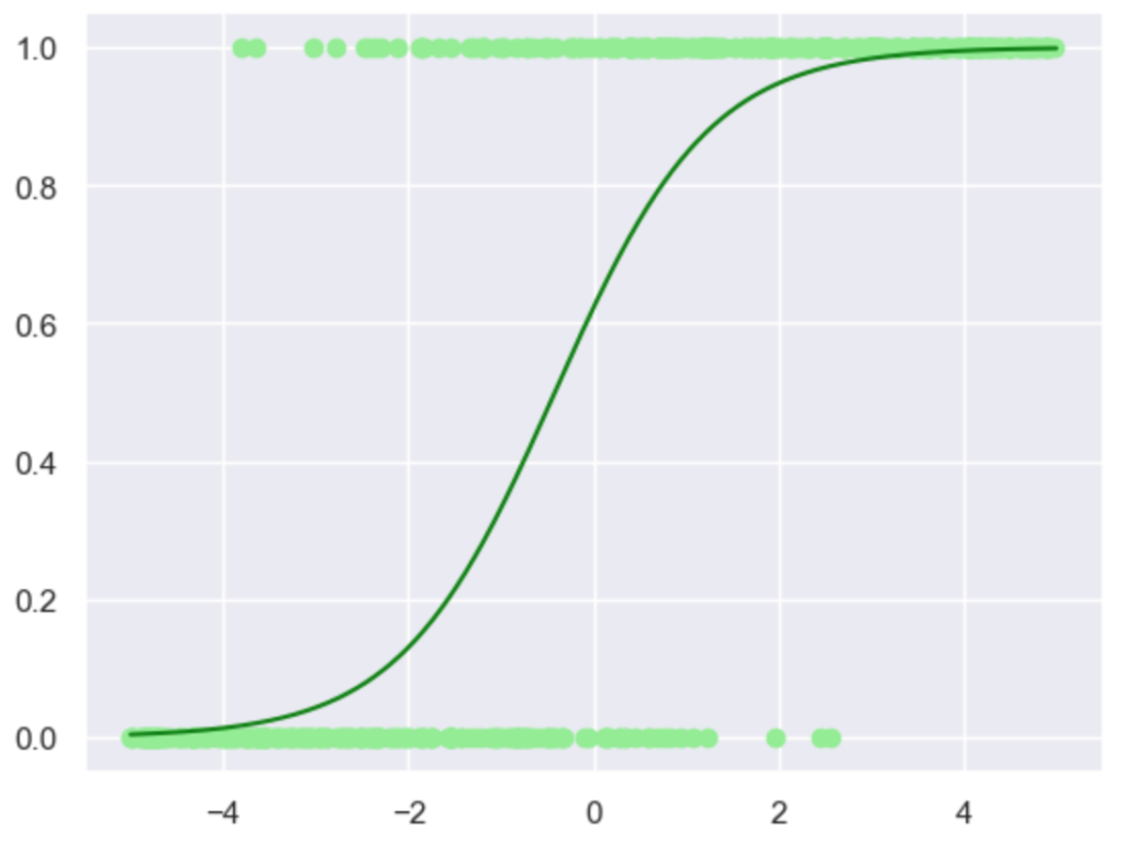
上記に対し、下記を実行することで自動微分と勾配法に基づいてパラメータ推定を行うことができる。
alpha = 0.01
a, b = 0.5, 0.

mul_coef_layer = MulLayer()
add_bias_layer = AddLayer()
calc_Sigmoid = Sigmoid()

for i in range(100):
    # forward
    u1 = mul_coef_layer.forward(x, a)
    u2 = add_bias_layer.forward(u1, b)
    y = calc_Sigmoid.forward(u2)
    #loss = t*np.log(y) + (1-t)*np.log(1-y)

    # backward
    #dloss = 1.
    dy = t/y - (1-t)/(1-y)
    du2 = calc_Sigmoid.backward(dy)
    du1, db = add_bias_layer.backward(du2)
    dx, da = mul_coef_layer.backward(du1)

    a += alpha*np.sum(da)
    b += alpha*np.sum(db)
    if (i+1)%10==0:
        print(a,b)
・実行結果
1.110878642205875 0.6047959437112932
1.1110570172855048 0.6055201115906093
1.1110586396377382 0.6055267041766271
1.1110586544122127 0.6055267642136816
1.1110586545467607 0.6055267647604263
1.1110586545479861 0.6055267647654055
1.111058654547997 0.6055267647654506
1.1110586545479972 0.6055267647654511
1.1110586545479972 0.6055267647654511
1.1110586545479972 0.6055267647654511
サンプリングに用いたパラメータの値が$a=1.2, b=0.5$であるので、上記は概ね適切な結果であることが確認できる。
注意:当記事ではクロスエントロピー誤差関数の実装を行なっていないので、dy = t/y - (1-t)/(1-y)は出力層の微分の式を用いた。