
当記事では「数理計画入門(朝倉書店)」の読解サポートにあたってChapter.$4$の「非線形計画」の章末問題の解答の作成を行いました。
基本的には書籍の購入者向けの解説なので、まだ入手されていない方は購入の上ご確認ください。また、解説はあくまでサイト運営者が独自に作成したものであり、書籍の公式ページではないことにご注意ください。
・解答まとめ
https://www.hello-statisticians.com/answer_textbook_math_optimization#green
Contents
章末の演習問題について
問題4.1の解答例
問題4.2の解答例
$$
\large
\begin{align}
f(\mathbf{x}) = 4x_1^2 – 2x_1x_2 + x_2^2 – 10x_1 – 8x_2 – 100
\end{align}
$$
上記の勾配ベクトル$\nabla f(\mathbf{x})$は下記のように計算できる。
$$
\large
\begin{align}
\nabla f(\mathbf{x}) &= \left(\begin{array}{c} \displaystyle \frac{\partial f}{\partial x_1} \\ \displaystyle \frac{\partial f}{\partial x_2} \end{array} \right) \\
&= \left(\begin{array}{c} 8x_1 – 2x_2 – 10 \\ -2x_1 + 2x_2 – 8 \end{array} \right)
\end{align}
$$
同様にヘッセ行列$\nabla^{2} f(\mathbf{x})$は下記のように計算できる。
$$
\large
\begin{align}
\nabla^{2} f(\mathbf{x}) &= \left(\begin{array}{cc} \displaystyle \frac{\partial^2 f}{\partial x_1^2} & \displaystyle \frac{\partial^2 f}{\partial x_1 \partial x_2} \\ \displaystyle \frac{\partial^2 f}{\partial x_2 \partial x_1} & \displaystyle \frac{\partial^2 f}{\partial x_2^2} \end{array} \right) \\
&= \left(\begin{array}{cc} 8 & -2 \\ -2 & 2 \end{array} \right)
\end{align}
$$
問題4.3の解答例
$$
\large
\begin{align}
\mathrm{Objective} : \quad & f(\mathbf{x}) = -x_1^4-x_2^4-x_1x_2+4x_2 \, \rightarrow \, \mathrm{Minimize} \\
\mathrm{Constraint} : \quad & c_1(\mathbf{x}) = x_1^3-x_2 \leq 0 \\
& c_2(\mathbf{x}) = x_1^2+x_2^2-2 \leq 0 \\
& c_3(\mathbf{x}) = -x_1 \leq 0
\end{align}
$$
$[a]$
import numpy as np
import matplotlib.pyplot as plt

r = np.sqrt(2)
theta = np.linspace(0,2*np.pi,100)
x_r = np.arange(0., 1.01, 0.01)

plt.plot(np.arange(-1.2,1.21,0.01), np.arange(-1.2,1.21,0.01)**3, "k--")
plt.plot(r*np.cos(theta),r*np.sin(theta),"k--")
plt.plot(np.arange(-1.7,1.71,0.01)*0, np.arange(-1.7,1.71,0.01), "k--")

plt.fill_between(x_r, x_r**3, np.sqrt(2-x_r**2), color="lightgreen")
plt.scatter([1., 0., 0.], [1., np.sqrt(2), 0.], marker="*", s=500, color="blue")

plt.show()
・実行結果
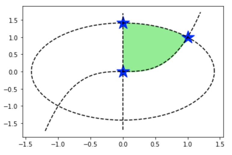
上図より$\mathbf{a}$〜$\mathbf{c}$が全て実行可能解であることが確認できる。また、有効制約は$\mathbf{a}$が$c_1$と$c_2$、$\mathbf{b}$が$c_2$と$c_3$、$\mathbf{c}$が$c_1$と$c_3$であることも同時に確認できる。