当記事は「基礎統計学Ⅰ 統計学入門(東京大学出版会)」の読解サポートにあたってChapter.13の「回帰分析」の章末問題の解説について行います。
※ 基本的には書籍の購入者向けの解説なので、まだ入手されていない方は下記より入手をご検討ください。また、解説はあくまでサイト運営者が独自に作成したものであり、書籍の公式ページではないことにご注意ください。(そのため著者の意図とは異なる解説となる可能性はあります)
・解答まとめ
https://www.hello-statisticians.com/answer_textbook_stat_basic_1-3#red
章末の演習問題について
問題13.1の解答例
i)
下記を実行することで散布図を作成することができる。
import numpy as np
import matplotlib.pyplot as plt

x = np.array([2., 2., 2., 2., 2.5, 2.5, 2.5, 2.5, 2.5, 2.5, 3., 3., 3., 3., 3., 3., 3., 3.5, 3.5, 3.5, 3.5, 3.5, 3.5, 4., 4., 4., 4., 4., 4., 4., 4.5, 4.5, 4.5, 4.5, 4.5, 4.5, 5., 5., 5., 5., 5., 5., 5.5, 5.5, 5.5, 5.5, 5.5, 5.5, 6., 6., 6., 6., 6., 6.5, 6.5, 6.5, 6.5, 7.])
y = np.array([2., 2.5, 2.5, 3., 2., 2.5, 3., 3., 3., 3.5, 2.5, 3., 3., 3.5, 3.5, 4., 4.5, 3., 3.5, 4., 4.5, 5., 5.5, 3.5, 4., 4.5, 4.5, 5., 5.5, 5.5, 4., 4.5, 5., 5., 5.5, 5.5, 6., 4.5, 5., 5.5, 6., 6.5, 5., 5.5, 5.5, 6., 6.5, 7., 5.5, 5.5, 6., 6.5, 7., 5.5, 6.5, 7., 7., 7.5])

plt.scatter(x,y)
plt.show()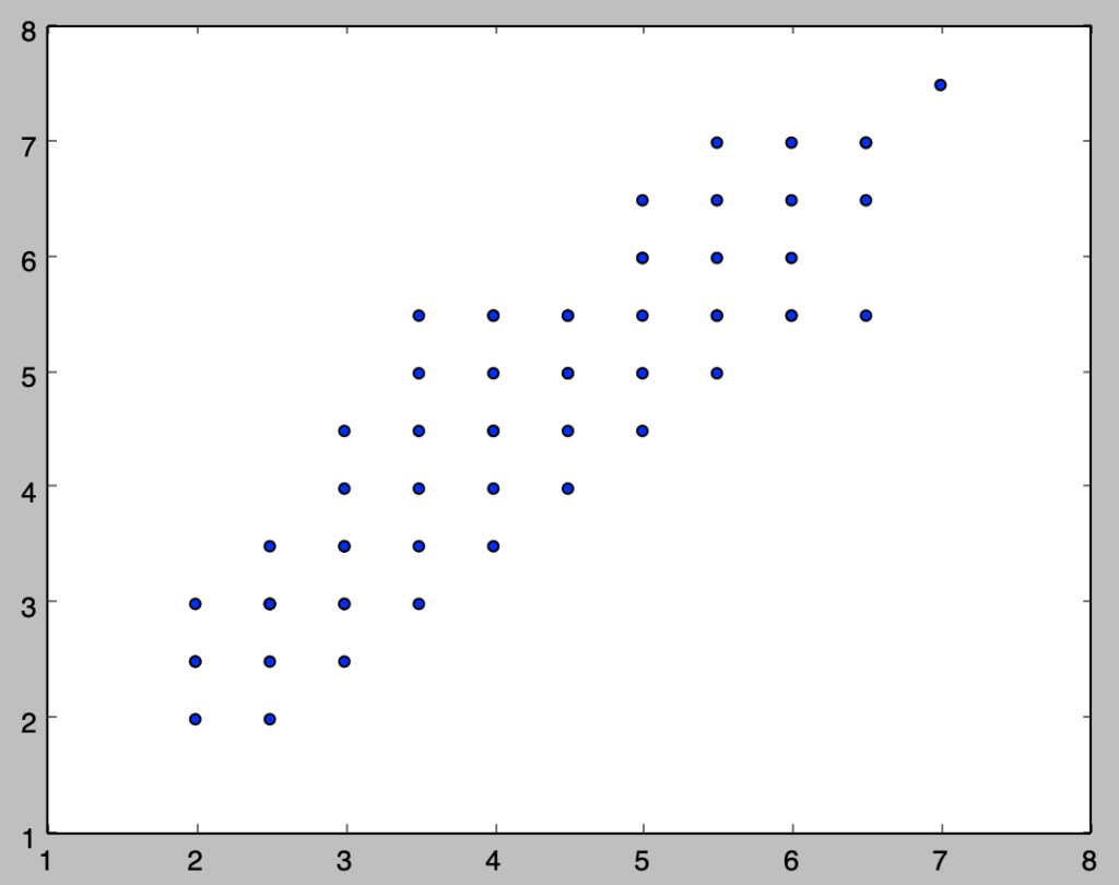
ⅱ)
$y_i = \beta_{0} + \beta_{1} x_i$のように回帰式を定義したとき、係数の$\beta_{0}, \beta_{1}$は下記を実行することで計算できる。
import numpy as np
import matplotlib.pyplot as plt

beta = np.zeros(2)
x_ = np.arange(1., 8., 0.1)

x = np.array([2., 2., 2., 2., 2.5, 2.5, 2.5, 2.5, 2.5, 2.5, 3., 3., 3., 3., 3., 3., 3., 3.5, 3.5, 3.5, 3.5, 3.5, 3.5, 4., 4., 4., 4., 4., 4., 4., 4.5, 4.5, 4.5, 4.5, 4.5, 4.5, 5., 5., 5., 5., 5., 5., 5.5, 5.5, 5.5, 5.5, 5.5, 5.5, 6., 6., 6., 6., 6., 6.5, 6.5, 6.5, 6.5, 7.])
y = np.array([2., 2.5, 2.5, 3., 2., 2.5, 3., 3., 3., 3.5, 2.5, 3., 3., 3.5, 3.5, 4., 4.5, 3., 3.5, 4., 4.5, 5., 5.5, 3.5, 4., 4.5, 4.5, 5., 5.5, 5.5, 4., 4.5, 5., 5., 5.5, 5.5, 6., 4.5, 5., 5.5, 6., 6.5, 5., 5.5, 5.5, 6., 6.5, 7., 5.5, 5.5, 6., 6.5, 7., 5.5, 6.5, 7., 7., 7.5])

beta[1] = np.sum((x-np.mean(x))*(y-np.mean(y)))/np.sum((x-np.mean(x))**2)
beta[0] = np.mean(y) - beta[1]*np.mean(x)

print("beta_0: {:.3f}, beta_1:{:.3f}".format(beta[0], beta[1]))

plt.scatter(x, y, color="green")
plt.plot(x_, beta[0]+beta[1]*x_)
plt.show()
・実行結果
> print("beta_0: {:.3f}, beta_1:{:.3f}".format(beta[0], beta[1]))
beta_0: 0.726, beta_1:0.932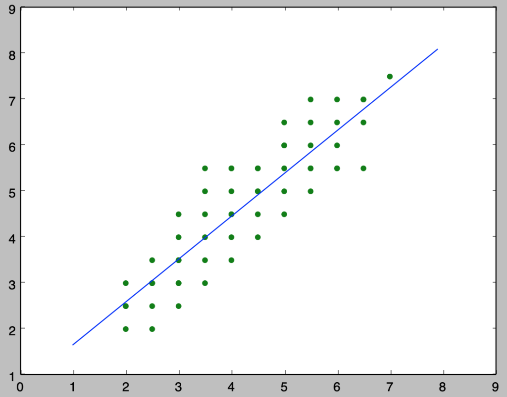
ⅲ)
$y_i = \beta_{0} + \beta_{1} x_i$のように考えるとき、推定結果と$(13.14), (13.16)$式より、回帰式の傾きに関する検定統計量$t$は下記のように計算できる。
$$
\large
\begin{align}
t &= \frac{\hat{\beta}_1-0.9}{s.e.(\hat{\beta}_1)} \quad (13.16) \\
s.e.(\hat{\beta}_1) &= \frac{\sqrt{\sum_{i=1}^{n} \hat{\epsilon}_{i}^{2}/n-2}}{\sqrt{\sum_{i=1}^{n} (x_i-\bar{x})^2}} \quad (13.14)
\end{align}
$$
ここで検定統計量$t$が自由度$n-2$の$t$分布$t(n-2)$に従うことを元に有意水準$5$%の検定を行えばよい。
上記に基づいて以下を実行することで結果を得ることができる。
import numpy as np
from scipy import stats

beta = np.zeros(2)

x = np.array([2., 2., 2., 2., 2.5, 2.5, 2.5, 2.5, 2.5, 2.5, 3., 3., 3., 3., 3., 3., 3., 3.5, 3.5, 3.5, 3.5, 3.5, 3.5, 4., 4., 4., 4., 4., 4., 4., 4.5, 4.5, 4.5, 4.5, 4.5, 4.5, 5., 5., 5., 5., 5., 5., 5.5, 5.5, 5.5, 5.5, 5.5, 5.5, 6., 6., 6., 6., 6., 6.5, 6.5, 6.5, 6.5, 7.])
y = np.array([2., 2.5, 2.5, 3., 2., 2.5, 3., 3., 3., 3.5, 2.5, 3., 3., 3.5, 3.5, 4., 4.5, 3., 3.5, 4., 4.5, 5., 5.5, 3.5, 4., 4.5, 4.5, 5., 5.5, 5.5, 4., 4.5, 5., 5., 5.5, 5.5, 6., 4.5, 5., 5.5, 6., 6.5, 5., 5.5, 5.5, 6., 6.5, 7., 5.5, 5.5, 6., 6.5, 7., 5.5, 6.5, 7., 7., 7.5])

beta[1] = np.sum((x-np.mean(x))*(y-np.mean(y)))/np.sum((x-np.mean(x))**2)
beta[0] = np.mean(y) - beta[1]*np.mean(x)

epsilon = y-(beta[0]+beta[1]*x)
s = np.sqrt(np.sum(epsilon**2)/(x.shape[0]-2.))

s_beta1 = s/np.sqrt(np.sum((x-np.mean(x))**2))
t = (beta[1]-0.9)/s_beta1

if t < stats.t.ppf(0.025,x.shape[0]-2) or stats.t.ppf(0.975,x.shape[0]-2) < t:
    print("t: {:.3f}, {} H_0".format(t,"reject"))
else:
    print("t: {:.3f}, {} H_0".format(t,"accept"))
・実行結果
t: 0.513, accept H_0上記より、帰無仮説$H_0: \beta_{1}=0.9$は棄却されない。
iv)
推定値$\hat{y}_i$に対する誤差項$\hat{\epsilon}_i$の分散の推定量を$s^2$とおき、$(13.8)$式の$\displaystyle s^2 = \sum_{i=1}^{n} \frac{\hat{\epsilon}_{i}^{2}}{n-2}$を計算し、$2s.e.$以上の外れ値があるかの確認を行う。
計算にあたっては以下を実行すれば良い。
import numpy as np

beta = np.zeros(2)

x = np.array([2., 2., 2., 2., 2.5, 2.5, 2.5, 2.5, 2.5, 2.5, 3., 3., 3., 3., 3., 3., 3., 3.5, 3.5, 3.5, 3.5, 3.5, 3.5, 4., 4., 4., 4., 4., 4., 4., 4.5, 4.5, 4.5, 4.5, 4.5, 4.5, 5., 5., 5., 5., 5., 5., 5.5, 5.5, 5.5, 5.5, 5.5, 5.5, 6., 6., 6., 6., 6., 6.5, 6.5, 6.5, 6.5, 7.])
y = np.array([2., 2.5, 2.5, 3., 2., 2.5, 3., 3., 3., 3.5, 2.5, 3., 3., 3.5, 3.5, 4., 4.5, 3., 3.5, 4., 4.5, 5., 5.5, 3.5, 4., 4.5, 4.5, 5., 5.5, 5.5, 4., 4.5, 5., 5., 5.5, 5.5, 6., 4.5, 5., 5.5, 6., 6.5, 5., 5.5, 5.5, 6., 6.5, 7., 5.5, 5.5, 6., 6.5, 7., 5.5, 6.5, 7., 7., 7.5])

beta[1] = np.sum((x-np.mean(x))*(y-np.mean(y)))/np.sum((x-np.mean(x))**2)
beta[0] = np.mean(y) - beta[1]*np.mean(x)

epsilon = y-(beta[0]+beta[1]*x)
s = np.sqrt(np.sum(epsilon**2)/(x.shape[0]-2.))

for i in range(x.shape[0]):
    if 2*s-np.abs(epsilon[i])<0:
        print("Outlier: Idx {} ({},{})".format(i+1,x[i],y[i]))
・実行結果
Outlier: Idx 23 (3.5,5.5)上記より$2s.e.$以上の外れ値が存在することが確認できる。
v)
ⅱ)で計算したbeta[0]とbeta[1]を用いて、下記を実行すれば良い。
print(beta[0]+beta[1]*8.)・実行結果
> print(beta[0]+beta[1]*8.)
8.18575023592
問題13.2の解答例
i)
下記を実行することで、散布図を作成することができる。
import numpy as np
import matplotlib.pyplot as plt

x = np.array([229., 367., 301., 352., 457., 427., 485., 616., 695., 806., 815., 826., 951., 1202., 881., 827., 1050., 1127., 1241., 1330., 1158., 1254., 1243., 1216., 1368., 1231., 1219., 1284., 1355.])
y = np.array([61.2, 70.0, 74.9, 82.8, 93.6, 98.5, 108.8, 120.1, 135.1, 152.5, 165.8, 173.0, 189.9, 202.6, 199.7, 205.0, 214.9, 226.3, 238.1, 250.7, 261.4, 271.0, 279.3, 288.4, 303.0, 317.3, 325.7, 340.3, 359.5])

plt.scatter(x,y)
plt.show()
・実行結果
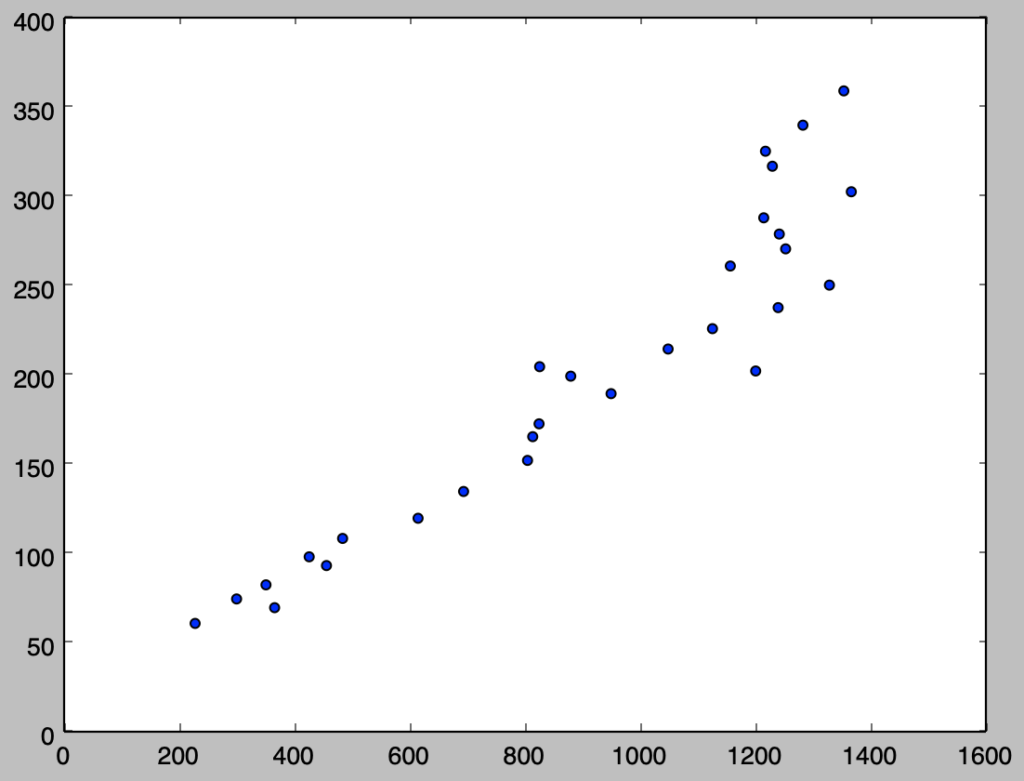
上記より、概ね正の相関があると考えることができる。
ⅱ)
下記を実行することで弾性値を推定することができる。
import numpy as np

beta = np.zeros(2)

x = np.array([61.2, 70.0, 74.9, 82.8, 93.6, 98.5, 108.8, 120.1, 135.1, 152.5, 165.8, 173.0, 189.9, 202.6, 199.7, 205.0, 214.9, 226.3, 238.1, 250.7, 261.4, 271.0, 279.3, 288.4, 303.0, 317.3, 325.7, 340.3, 359.5])
y = np.array([229., 367., 301., 352., 457., 427., 485., 616., 695., 806., 815., 826., 951., 1202., 881., 827., 1050., 1127., 1241., 1330., 1158., 1254., 1243., 1216., 1368., 1231., 1219., 1284., 1355.])

log_x = np.log(x)
log_y = np.log(y)

beta[1] = np.sum((log_x-np.mean(log_x))*(log_y-np.mean(log_y))) / np.sum((log_x-np.mean(log_x))**2)
beta[0] = np.mean(log_y) - beta[1]*np.mean(log_x)

print("Estimated beta_1: {:.3f}".format(beta[1]))
・実行結果
> print("Estimated beta_1: {:.3f}".format(beta[1]))
Estimated beta_1: 0.967
ⅲ)
ratio = 1.04**12
y_pred = 1355.*ratio*beta[1]

print(y_pred)
・実行結果
> print(y_pred)
2097.52451479
上記は巻末の解答とは異なる結果だが詳細の計算方法がわからないので、それほど大きく異ならないことからここでは許容した。
iv)
推定結果と$(13.14), (13.16)$式より、回帰式の傾きに関する検定統計量$t$は下記のように計算できる。
$$
\large
\begin{align}
t &= \frac{\hat{\beta}_1-1}{s.e.(\hat{\beta}_1)} \quad (13.16) \\
s.e.(\hat{\beta}_1) &= \frac{\sqrt{\sum_{i=1}^{n} \hat{\epsilon}_{i}^{2}/n-2}}{\sqrt{\sum_{i=1}^{n} (x_i-\bar{x})^2}} \quad (13.14)
\end{align}
$$
ここで検定統計量$t$が自由度$n-2$の$t$分布$t(n-2)$に従うことを元に帰無仮説$H_0: \beta_{1}=1$に対し、有意水準$5$%の検定を行えばよい。
上記に基づいて以下を実行することで結果を得ることができる。
import numpy as np
from scipy import stats

beta = np.zeros(2)

x = np.array([61.2, 70.0, 74.9, 82.8, 93.6, 98.5, 108.8, 120.1, 135.1, 152.5, 165.8, 173.0, 189.9, 202.6, 199.7, 205.0, 214.9, 226.3, 238.1, 250.7, 261.4, 271.0, 279.3, 288.4, 303.0, 317.3, 325.7, 340.3, 359.5])
y = np.array([229., 367., 301., 352., 457., 427., 485., 616., 695., 806., 815., 826., 951., 1202., 881., 827., 1050., 1127., 1241., 1330., 1158., 1254., 1243., 1216., 1368., 1231., 1219., 1284., 1355.])

log_x = np.log(x)
log_y = np.log(y)

beta[1] = np.sum((log_x-np.mean(log_x))*(log_y-np.mean(log_y))) / np.sum((log_x-np.mean(log_x))**2)
beta[0] = np.mean(log_y) - beta[1]*np.mean(log_x)

epsilon = log_y-(beta[0]+beta[1]*log_x)
s = np.sqrt(np.sum(epsilon**2)/(x.shape[0]-2.))

s_beta1 = s/np.sqrt(np.sum((log_x-np.mean(log_x))**2))
t = (beta[1]-1.)/s_beta1

if t < stats.t.ppf(0.025,x.shape[0]-2) or stats.t.ppf(0.975,x.shape[0]-2) < t:
    print("t: {:.3f}, {} H_0".format(t,"reject"))
else:
    print("t: {:.3f}, {} H_0".format(t,"accept"))
・実行結果
t: -0.725, accept H_0上記より、帰無仮説$H_0: \beta_{1}=1$は棄却されない。
[…] 詳しくは下記などでも取り扱いを行った。https://www.hello-statisticians.com/explain-books-cat/toukeigakunyuumon-akahon/ch13_practice.html […]