
当記事は「基礎統計学Ⅲ 自然科学の統計学(東京大学出版会)」の読解サポートにあたってChapter.$7$の「分布の仮定」の章末問題の解説について行います。
基本的には書籍の購入者向けの解答例・解説なので、まだ入手されていない方は下記より入手をご検討ください。また、解説はあくまでサイト運営者が独自に作成したものであり、書籍の公式ページではないことにご注意ください。

https://www.amazon.co.jp/dp/4130420674
章末の演習問題について
問題7.1の解答例
問題7.2の解答例
i)
$$
\large
\begin{align}
L(\theta) = \sum_{i=1}^{n} (X_i-\theta)^2
\end{align}
$$
上記のような$L(\theta)$が与えられたとき、$L(\theta)$を最小にする$\theta$を考える。
ここで$L(\theta)$を$\theta$で微分すると下記が得られる。
$$
\large
\begin{align}
\frac{\partial L(\theta)}{\partial \theta} &= -2 \sum_{i=1}^{n} (X_i-\theta) \\
&= -2 (n \bar{X} – n \theta) \\
&= 2n (\theta – \bar{X})
\end{align}
$$
上記は$\theta$の単調増加関数であることから、$L(\theta)$を最小にする$\theta$は$\bar{X}$であることがわかる。
問題7.3の解答例
下記のPython実装のような計算を行うことで、結果を計算することができる。
import numpy as np

x = np.array([8.2,7.5,8.7,8.4,9.6])
theta = 8.4
for i in range(10):
    W = 1/(1+(x-theta)**2)
    theta = np.sum(W*x)/np.sum(W)
    print(theta)
・実行結果
8.42017221731
8.42650412892
8.42849591517
8.42912290722
8.42932032277
8.42938248582
8.42940206044
8.42940822436
8.42941016535
8.42941077656
問題7.4の解答例
i)
観測値は下記のように幹葉表示することができる。
$$
\large
\begin{array}{|c|*3{c|}}\hline \mathrm{stem} & \mathrm{leaf} & \mathrm{degree} & \mathrm{depth} : n=25 \\
\hline 5.5 & 77 & 2 & 2 \\
\hline 5.2 & 5 & 1 & 3 \\
\hline 5.1 & 233689 & 6 & 9 \\
\hline 5.0 & 112458 & 6 & \\
\hline 4.9 & 058 & 3 & 10 \\
\hline 4.8 & 0117 & 4 & 7 \\
\hline 4.7 & 9 & 1 & 3 \\
\hline 4.6 & 9 & 1 & 2 \\
\hline 4.5 & 8 & 1 & 1 \\
\hline
\end{array}
$$
ⅱ)
下記のPythonを実行することで平均$\bar{X}$が得られる。
import numpy as np

x = np.array([4.95,5.02,5.08,4.90,5.12,5.19,4.80, \
4.87,4.98,4.58,4.81,5.18,5.25,5.05,4.79,5.57,5.01, \
5.57,5.01,4.81,5.13,5.04,5.13,5.16,4.69])

print(np.sum(x)/25.)
・実行結果
5.0276ⅲ)
i)で表した幹葉表示より、$X_{med}=5.02$であることが確認できる。
iv)
下記のPythonを実行することで$k=3$のトリム平均$\hat{\theta}_{trim}(3)$が得られる。
import numpy as np

x = np.array([4.95,5.02,5.08,4.90,5.12,5.19,4.80, \
4.87,4.98,4.58,4.81,5.18,5.25,5.05,4.79,5.57,5.01, \
5.57,5.01,4.81,5.13,5.04,5.13,5.16,4.69])

print(np.sum(np.sort(x)[3:-3])/(25.-6.))
・実行結果
5.0126...v)
vi)
問題7.5の解答例
$(7.33), (7.34)$式を元に二項分布$Bin(17,0.5)$を考えると、棄却域が$N \leq 4, 13 \leq N$のときに有意水準が$\alpha=0.0490 \simeq 0.05$となる。ここで与えられた観測値は$N=5$であるので、「母平均$=0$」の帰無仮説は棄却されない。
問題7.6の解答例
下記のように$2$つの標本を小さいものから順に並べることができる。第$2$標本の方が数が少ないので第$2$標本を元に考えるにあたって、第$2$標本の観測値には下線を引いた。
$$
\large
\begin{align}
& 42.6, 43.9, 44.1, 44.2, \underline{44.7}, 45.0, 45.8, \underline{46.8}, \underline{46.9}, \underline{47.1}, \\
& 47.4, 48.0, \underline{48.2}, 48.7, 49.5, 49.6, \underline{50.0}, 50.0, 51.4, \underline{52.1}, \\
& 52.7, 52.8, \underline{53.5}, \underline{54.2}, \underline{56.3}
\end{align}
$$
上記より、第$2$標本の各観測値の順位はそれぞれ下記のように表される。
$$
\large
\begin{align}
5, 8, 9, 10, 13, 17.5, 20, 23, 24, 25
\end{align}
$$
従って、順位和$W$は$W=154.5$となる。本文の表$7.2$より、両側$5%$の棄却域は$94$以下または$m(m+n+1)-94=10(10+15+1)-94=166$以上である。よって、「二つの平均が等しい」と考える帰無仮説は棄却できない。
問題7.7の解答例
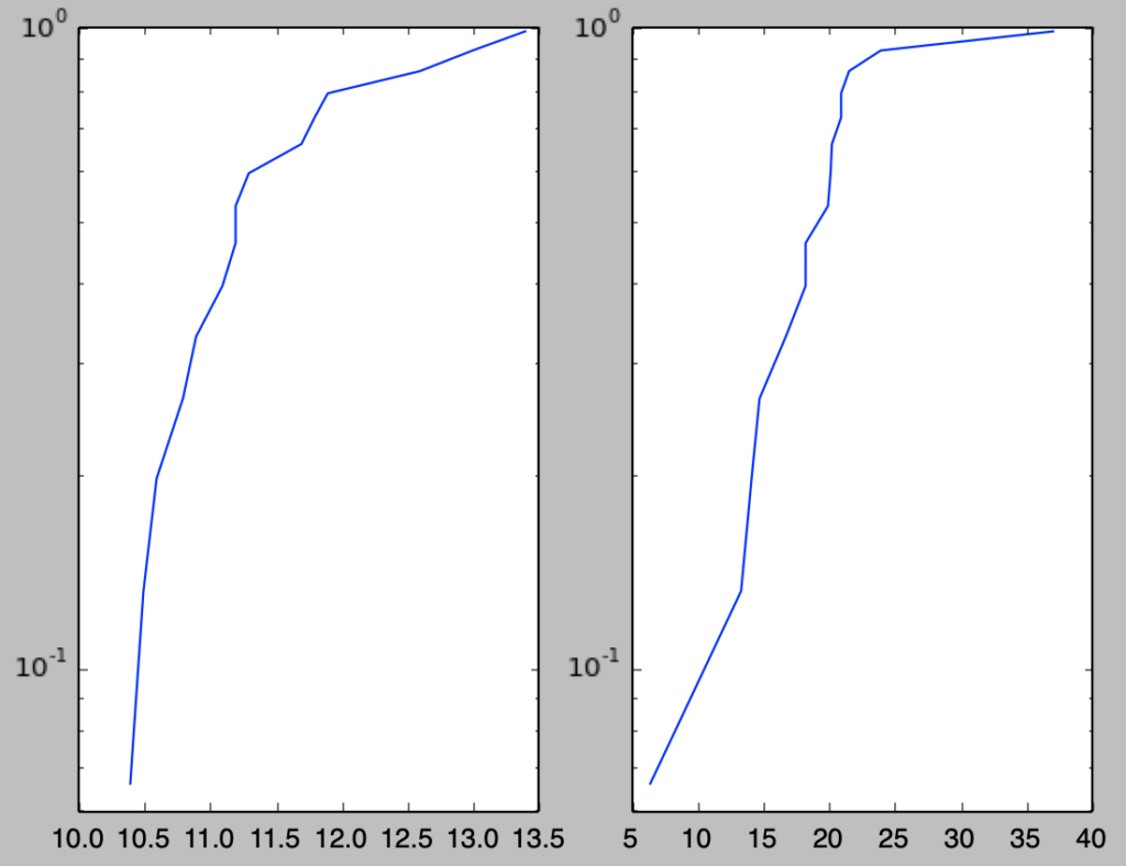
i)
下記を実行することで正規確率紙へのプロットを行うことができる。
import numpy as np
import matplotlib.pyplot as plt

x_A = np.array([10.5, 10.4, 10.6, 11.9, 11.3, 11.8, 11.7, 12.6, 10.9, 11.1, 13.0, 11.2, 13.4, 10.8, 11.2])
x_B = np.array([20.0, 18.3, 20.3, 37.1, 20.2, 21.0, 6.5, 24.0, 14.2, 21.0, 18.3, 13.4, 14.8, 21.6, 16.8])

x_A_ranked = np.sort(x_A)
x_B_ranked = np.sort(x_B)
y = np.linspace(0.,1.,16)

plt.subplot(121)
plt.plot(x_A_ranked,y[1:])
plt.yscale("log")
plt.ylim([0.06,1.01])
plt.subplot(122)
plt.plot(x_B_ranked,y[1:])
plt.yscale("log")
plt.ylim([0.06,1.01])
plt.show()
・実行結果
ⅱ)
下記を実行することで$b_1, b_2$の計算を行うことができる。
def calc_moment(x):
    m2 = np.sum((x-np.mean(x))**2)/x.shape[0]
    m3 = np.sum((x-np.mean(x))**3)/x.shape[0]
    m4 = np.sum((x-np.mean(x))**4)/x.shape[0]
    b1 = m3/(m2)**(1.5)
    b2 = m4/m2**2 - 3.
    return b1, b2

b1_A, b2_A = calc_moment(x_A)
b1_B, b2_B = calc_moment(x_B)

print("・A")
print("b1: {:.2f}, b2: {:.2f}".format(b1_A,b2_A))
print("===")
print("・B")
print("b1: {:.2f}, b2: {:.2f}".format(b1_B,b2_B))
・実行結果
・A
b1: 0.80, b2: -0.40
===
・B
b1: 0.90, b2: 2.40
ここで$n=15$のときの$5%$点が$b_1=0.9, b_2=1.1$、$1$%点が$b_1=1.3, b_2=2.3$であることから、$A$は$5$%でも棄却できず、$B$は$1$%で棄却できることが確認される。よって、$B$は正規分布に従っていないと考えられる。